Programming Languages

Jump to Section

Programming Languages as taught by William Hawkins III

pdf version is here

conversion didn’t go as well as I hoped, but the jupyter notebook version is here. Need to look into more pandoc stuff.

8/23/2021

Definitions:

programming language: A system of communicating computational ideas between people and computing machines.
high-level programming language: A programming language that is independent of any particular machine architecture.
syntax: The rules for constructing structurally valid (note: valid, not correct) computer programs in a particular language.
names: A means of identifying “entities” in a programming language.
types: A type denotes the kinds of values that a program can manipulate. (A more specific definition will come later in the course).
semantics: The effect of each statement’s execution on the program’s operation.

Concepts:

There are four fundamental components of every programming language: syntax, names, types, and semantics.

Practice:

For your favorite programming language, attempt to explain the most meaningful parts of its syntax. Think about what are valid identifiers in the language, how statements are separated, whether blocks of code are put inside braces, etc.
Next, ask yourself how your favorite language handles types. Are variables in the language given types explicitly or implicitly? If the language is compiled, are types assigned to variables before the code is compiled or as the program executes? These are issues that we will discuss in detail in Module 2.
Finally, think about how statements in your favorite programming language affect the program’s execution. Does the language have loops? if-then statements? function composition? goto?

8/25/2021

The value of studying PLs

Every new language that you learn gives you new ways to think about and solve problems.
1. There is a parallel here with natural languages.
2. Certain written/spoken languages have words for concepts that others do not.
3. Linguists have said that people can only conceive ideas for which there are words.
4. In certain programming languages there may be constructs (“words”) that give you a power to solve problems and write algorithms in new, interesting ways.
You can choose the right tool for the job.
- When all you have is a hammer, everything looks like a nail.
Makes you an increasingly flexible programmer.
- The more you know about the concepts of programming languages (and the PLs that you know) the easier it is to learn new languages.
Using PLs better Studying PLs will teach you about how languages are implemented. This “awareness” can give you insight into the “right way” to do something in a particular language. For instance, if you know that recursion and looping are equally performant and computationally powerful, you can choose to use the one that improves the readability of your code. However, if you know that iteration is faster (and that’s important for your application) then you will choose that method for invoking statements repeatedly.

Programming domains

We write programs to solve real-world problems.
The problems that we are attempting to solve lend themselves to programming languages with certain characteristics.
Some of those real-world problems are related to helping others solve real-world problems (systems programs):
- e.g., operating systems, utilities, compilers, interpreters, etc.
- There are a number of good languages for writing these applications: C, C++, Rust, Python, Go, etc.
But, most of programs are designed/written to solve actually real-world problems:
- scientific calculations: these applications need to be fast (parallel?) and mathematically precise (work with numbers of many kinds). Scientific applications were the earliest programming domain and inspired the first high-level programming language, Fortran.
- artificial intelligence: AI applications manipulate symbols (in particular, lists of symbols) as opposed to numbers. This application requirement gave rise to a special type of language designed especially for manipulating lists, Lisp (List Processor).
- world wide web: WWW applications must embed code in data (HTML). Because of how WWW applications advance so quickly, it is important that languages for writing these applications support rapid iteration. Common languages for writing web applications are PERL, Python, JavaScript, Ruby, Go, etc.
- business: business applications need to produce reports, process character-based data, describe and store numbers with specific precision (aka, decimals). COBOL has traditionally been the language of business applications, although new business applications are being written in other languages these days (Java, the .Net languages).
- machine learning: machine learning applications require sophisticated math and algorithms and most developers do not want to rewrite these when good alternatives are available. For this reason, a language with a good ecosystem of existing libraries makes an ideal candidate for writing ML programs (Python).
- game development: So-called AAA games must be fast enough to generate lifelike graphics and immersive scenes in near-real time. For this reason, games are often written in a language that is expressive but generates code that is optimized, C++.

This list is non-exhaustive, obviously!

The John von Neumann Model of Computing

This computing model has had more influence on the development of PLs than we can imagine.
There are two hardware components in this Model (the processor [CPU] and the memory) and they are connected by a pipe.
- The CPU pipes data and instructions (see below) to/from the memory (fetch).
- The CPU reads that data to determine the action to take (decode).
- The CPU performs that operation (execute).
- Because there is only one path between the CPU and the memory, the speed of the pipe is a bottleneck on the processor’s efficiency.
The Model is interesting because of the way that it stores instructions and data together in the same memory.
It is different than the Harvard Architecture where programs and data are stored in different memory.
In the Model, every bit of data is accessible according to its address.
Sequential instructions are placed nearby in memory.
- For instance, in

for (int i = 0; i < 100; i++) {
  statement1;
  statement2;
  statement3;
}

statement1, statement2 and statement3 are all stored one after the other in memory.

Modern implementations of the Model make fetching nearby data fast.
Therefore, implementing repeated instructions with loops is faster than implementing repeated loops with recursion.
Or is it?
This is a particular case where learning about PL will help you as a programmer!

8/27/2021

Programming Paradigms

A paradigm is a pattern or model. A programming paradigm is a pattern of problem-solving thought that underlies a particular genre of programs and languages.
- According to their syntax, names and types, and semantics, it is possible to classify languages into one of four categories (imperative, object-oriented, functional and logic).
- That said, modern researchers in PL are no longer as convinced that these are meaningful categories because new languages are generally a collection of functionality and features and contain bits and pieces from each paradigm.
The paradigms:
1. Imperative: Imperative languages are based on the centrality of assignment statements to change program state, selection statements to control program flow, loops to repeat statements and procedures for process abstraction (a term we will learn later).
  - These languages are most closely associated with the von Neumann architecture, especially assignment statements that approximate the piping operation at the hardware level.
  - Examples of imperative languages include C, Fortran, Cobol, Perl.
2. Object-oriented: Object-oriented languages are based upon a combination of data abstraction, data hiding, inheritance and message passing.
  - Objects respond to messages by modifying their internal data – in other words, they become active.
  - The power of inheritance is that an object can reuse an implementation without having to rewrite the code.
  - These languages, too, are closely associated with the von Neumann architecture and (usually) inherit selection statements, assignment statements and loops from imperative programming languages. Examples of object-oriented languages include Smalltalk, Ruby, C++, Java, Python, JavaScript.
3. Functional: Functional programming languages are based on the concept that functions are first-class objects in the language – in other words, functions are just another type like integers, strings, etc.
  - In a functional PL, functions can be passed to other functions as parameters and returned from functions.
  - The loops and selection statements of imperative programming languages are replaced with composition, conditionals, and recursion in functional PLs.
  - A subset of functional PLs are known as pure functional PLs because functions those languages have no side-effects (a side-effect occurs in a function when that function performs a modification that can be seen outside the function – e.g., changing a value of a parameter, changing a global variable, etc).
  - Examples of functional languages include Lisp, Scheme, Haskell, ML, JavaScript, Python.
4. Logic: Simply put, logic programming languages are based on describing what to compute and not how to compute it.
  - Prolog (and its variants) are really the only logic programming language in widespread use.

Language Evaluation Criteria (New Material Alert)

There are four (common) criteria for evaluating a programming language:

Readability: A metric for describing how easy/hard it is to comprehend the meaning of a computer program written in a particular language.
1. Overall simplicity: The number of basic concepts that a PL has.
  1. Feature multiplicity: Having more than one way to accomplish the same thing.
  2. Operator overloading: Operators perform different computation depending upon the context (i.e., the type of the operands)
  3. Simplicity can be taken too far. Consider machine language.
2. Orthogonality: How easy/hard it is for the constructs of a language to be combined to build higher-level control and data structures.
  1. Alternate definition: The mutual independence of primitive operations.
  2. Orthogonal example: any type of entity in a language can be passed as a parameter to a function.
  3. Non-orthogonal example: only certain entities in a language can be used as a return value from a function (e.g., in C/C++ you cannot return an array).
  4. This term comes from the mathematical concept of orthogonal vectors where orthogonal means independent.
  5. The more orthogonal a language, the fewer exceptional cases there are in the language’s semantics.
  6. The more orthogonal a language, the slower the language: The compiler/interpreter must be able to compute based on every single possible combination of language constructs. If those combinations are restricted, the compiler can make optimizations and assumptions that will speed up program execution.
3. Data types: Data types make it easier to understand the meaning of variables.
  - e.g., the difference between int userHappy = 0; and bool userHappy = True;
4. Syntax design
  1. A PL’s reserved words should make things clear. For instance, it is easier to match the beginnings and endings of loops in a language that uses names rather than { }s.
  2. The PL’s syntax should evoke the operation that it is performing.
    1. For instance, a + should perform some type of addition operation (mathematical, concatenation, etc)
Writeability
1. Includes all the aspects of Readability, and
2. Expressiveness: An expressive language has relatively convenient rather than cumbersome way of specifying computations.
Reliability: How likely is it that a program written in a certain PL is correct and runs without errors.
1. Type checking: a language with type checking is more reliable than one without type checking; type checking is testing for operations that compute on variables with incorrect types at compile time or runtime.
  - Type checking is better done at runtime.
  - A strongly typed programming language is one that is always able to detect type errors either at compile time or runtime.
2. Exception handling (the ability of a program to intercept runtime errors and take corrective action) and aliasing (when two or more distinct names in a program point to the same resource) affect the PL’s reliability.
3. 1. 1. 1. In truth, there are so many things that affect the reliability of a PL.
4. The easier a PL is to read and write, the more reliable the code is going to be.
Cost: The cost of writing a program in a certain PL is a function of
1. The cost to train programmers to use that language
2. The cost of writing the program in that language
3. The time/speed of execution of the program once it is written
4. The cost of poor reliability
5. The cost of maintenance – most of the time spent on a program is in maintaining it and not developing it!

8/30/2021

Today we learned a more complete definition of imperative programming languages and studied the defining characteristics of variables. Unfortunately we did not get as far as I wanted during the class which means that there is some new material in this edition of the Daily PL!

Imperative Programming Languages

Any language that is an abstraction of the von Neumann Architecture can be considered an imperative programming language.

There are 5 calling cards of imperative programming languages:

state, assignment statements, and expressions: Imperative programs have state. Assignment statements are used to modify the program state with computed values from expressions
1. state: The contents of the computer’s memory as a program executes.
2. expression: The fundamental means of specifying a computation in a programming language. As a computation, they produce a value.
3. assignment statement: A statement with the semantic effect of destroying a previous value contained in memory and replacing it with a new value. The primary purpose of the assignment statement is to have a side effect of changing values in memory. As Sebesta says, “The essence of the imperative programming languages is the dominant role of the assignment statement.”
variables: The abstraction of the memory cell.
loops: Iterative form of repetition (for, while, do … while, foreach, etc)
selection statements: Conditional statements (if/then, switch, when)
procedural abstraction: A way to specify a process without providing details of how the process is performed. The primary means of procedural abstraction is through definition of subprograms (functions, procedures, methods).

Variables

There are 6 attributes of variables. Remember, though, that a variable is an abstraction of a memory cell.

type: Collection of a variable’s valid data values and the collection of valid operations on those values.
name: String of characters used to identify the variable in the program’s source code.
scope: The range of statements in a program in which a variable is visible. Using the yet-to-be-defined concept of binding, there is an alternative definition: The range of statements where the name’s binding to the variable is active.
lifetime: The period of time during program execution when a variable is associated with computer memory.
address: The place in memory where a variable’s contents (value) are stored. This is sometimes called the variable’s l-value because only a variable associated with an address can be placed on the left side of an assignment operator.
value: The contents of the variable. The value is sometimes call the variable’s r-value because a variable with a value can be used on the right side of an assignment operator.

Looking forward to Binding (New Material Alert)

A binding is an association between an attribute and an entity in a programming language. For example, you can bind an operation to a symbol: the + symbol can be bound to the addition operation.

Binding can happen at various times:

Language design (when the language’s syntax and semantics are defined or standardized)
Language implementation (when the language’s compiler or interpreter is implemented)
Compilation
Loading (when a program [either compiled or interpreted] is loaded into memory)
Execution

A static binding occurs before runtime and does not change throughout program execution. A dynamic binding occurs at runtime and/or changes during program execution.

Notice that the six “things” we talked about that characterize variables are actually attributes!! In other words, those attributes have to be bound to variables at some point. When these bindings occur is important for users of a programming language to understand. We will discuss this on Wednesday! blob:https://1492301-4.kaf.kaltura.com/903896d9-2341-4dd3-9709-ca344de08719

9/1/2021

Welcome to the Daily PL for September 1st, 2021! As we turn the page from August to September, we started the month discussing variable lifetime and scope. Lifetime is related to the storage binding and scope is related to the name binding. Before we learned that new material, however, we went over an example of the different bindings and their times in an assignment statement.

Binding Example

Consider a Python statement like this:

vrb = arb + 5

Recall that a binding is an association between an attribute and an entity. What are some of the possible bindings (and their times) in the statement above?

The symbol + (entity) must be bound to an operation (attribute). In a language like Python, that binding can only be done at runtime. In order to determine whether the operation is a mathematical addition, a string concatenation or some other behavior, the interpreter needs to know the type of arb which is only possible at runtime.
The numerical literal 5 (entity) must be bound to some in-memory representation (attribute). For Python, it appears that the interpreter chooses the format for representing numbers in memory (https://docs.python.org/3/library/sys.html#sys.int%5Finfo (Links to an external site.), https://docs.python.org/3/library/sys.html#sys.float%5Finfo (Links to an external site.)) which means that this binding is done at the time of language implementation.
The value (attribute) of the variables vrb and arb (entities) are bound at runtime. Remember that the value of a variable is just another binding.

This is not an exhaustive list of the bindings that are active for this statement. In particular, the variables vrb and arb must be bound to some address, lifetime and scope. Discussing those bindings requires more information about the statement’s place in the source code.

Variables’ Storage Bindings

The storage binding is related to the variable’s lifetime (the time during which a variable is bound to memory). There are four common lifetimes:

static: Variable is bound to storage before execution and remains bound to the same storage throughout program execution.
1. Variables with static storage binding cannot share memory with other variables (they need their storage throughout execution).
2. Variables with static storage binding can be accessed directly (in other words, their access does not require redirection through a pointer) because the address of their storage is constant throughout execution. Direct addressing means that accesses are faster.
3. Storage for variables with static binding does not need to be repeatedly allocated and deallocated throughout execution – this will make program execution faster.
4. In C++, variables with static storage binding are declared using the static keyword inside functions and classes.
5. Variables with static storage binding are sometimes referred to as history sensitive because they retain their value throughout execution.
stack dynamic: Variable is bound to storage when it’s declaration statements are elaborated (the time when a declaration statement is executed).
1. Variables with stack dynamic storage bindings make recursion possible because their storage is allocated anew every time that their declaration is elaborated. To fully understand this point it is necessary to understand the way that function invocation is handled using a runtime stack. We will cover this topic next week. Stay tuned!
2. Variables with stack dynamic storage bindings cannot be directly accessed. Accesses must be made through an intermediary which makes them slower. Again, this will make more sense when we discuss the typical mechanism for function invocation.
3. The storage for variables with stack dynamic storage bindings are constantly allocated and deallocated which adds to runtime overhead.
Variables with stack dynamic storage bindings are not history sensitive.
Explicit heap dynamic: Variable is bound to storage by explicit instruction from the programmer. E.g., new / malloc in C/C++.
1. The binding to storage is done at runtime when these explicit instructions are executed.
2. The storage sizes can be customized for the use.
3. The storage is hard to manage and requires careful attention from the programmer.
4. The storage for variables with explicit heap dynamic storage bindings are constantly allocated and deallocated which adds to runtime overhead.
Implicit heap dynamic: Variable is bound to storage when it is assigned a value at runtime.
1. All storage bindings for variables in Python are handled in this way. https://docs.python.org/3/c-api/memory.html (Links to an external site.)
2. When a variable with implicit heap dynamic storage bindings is assigned a value, storage for that variable is dynamically allocated.
3. Allocation and deallocation of storage for variables with implicit heap dynamic storage bindings is handled automatically by the language compiler/interpreter. (More on this when we discuss memory management techniques in Module 3).

Variables’ Name Bindings

See the Pl for the Video.

This new material is presented above as Episode 1 of PL After Dark. Below you will find a written recap!

Scope is the range of statements in which a variable is visible (either referencable or assignable). Using the vocabulary of bindings, scope can also be defined as the collection of statements which can access a name binding. In other words, scope determines the binding of a name to a variable.

It is easy to get fooled into thinking that a variable’s name is intrinsic to the variable. However, a variable’s name is just another binding like address, storage, value, etc. There are two scopes that most languages employ:

local: A variable is locally scoped to a unit or block of a program if it is declared there. In Python, a variable that is the subject of an assignment is local to the immediate enclosing function definition. For instance, in

def add(a, b):
    total = a + b
    return total

total is a local variable.

global: A variable is globally scoped when it is not in any local scope (terribly unhelpful, isn’t it?) Using global variables breaks the principles of encapsulation and data hiding.

For a variable that is used that is not local, the compiler/interpreter must determine to which variable the name refers. Determining the name/variable binding can be done statically or dynamically:

Static Scoping

This is sometimes also known as lexical scoping. Static scoping is the type of scope that can be determined using only the program’s source code. In a statically scoped programming language, determining the name/variable binding is done iteratively by searching through a block’s nesting static parents. A block is a section of code with its own scope (in Python that is a function or a class and in C/C++ that is statements enclosed in a pair of {}s). The static parent of a block is the block in which the current block was declared. The list of static parents of a block are the block’s static ancestors.

Dynamic Scoping

Dynamic scoping is the type of scope that can be determined only during program execution. In a dynamically scoped programming language, determining the name/value binding is done iteratively by searching through a block’s nesting dynamic parents. The dynamic parent of a block is the block from which the current block was executed. Very few programming languages use dynamic scoping (BASH, PERL [optionally]) because it makes checking the types of variables difficult for the programmer (and impossible for the compiler/interpreter) and because it increases the “distance” between name/variable binding and use during program execution. However, dynamic binding makes it possible for functions to require fewer parameters because dynamically scoped non local variables can be used in their place.

9/3/2021

Welcome to The Daily PL for 9/3/2021. We spent most of Friday reviewing material from Episode 1 of PL After Dark and going over scoping examples in C++ and Python. Before continuing, make sure that you have viewed Episode 1 of PL After Dark.

Scope

We briefly discussed the difference between local and global scope.

It is easy to get fooled into thinking that a variable’s name is intrinsic to the variable. However, a variable’s name is just another binding like address, storage, value, etc.

As a programmer, when a variable is local determining the name/variable binding is straightforward. Determining the name/variable binding becomes more complicated (and more important) when source code uses a non-local name to reference a variable. In cases like this, determining the name/variable binding depends on whether the language is statically or dynamically scoped.

Static Scoping

This is sometimes also known as lexical scoping. Static scoping is the type of scope that can be determined using only the program’s source code. In a statically scoped programming language, determining the name/variable binding is done iteratively by searching through a block’s nesting static parents. A block is a section of code with its own scope (in Python that is a function or a class and in C/C++ that is statements enclosed in a pair of {}s). The static parent of a block is the block in which the current block was declared. The list of static parents of a block are the block’s static ancestors.

Here is pseudocode for the algorithm of determining the name/variable binding in a statically scoped programming language:

def resolve(name, current_scope) -> variable
  s = current_scope
  while (s != InvalidScope)
    if s.contains(name)
      return s.variable(name)
    s = s.static_parent_scope()
  return NameError

For practice doing name/variable binding in a statically scoped language, play around with an example in Python: static_scope.py

Consider this …

Python and C++ have different ways of creating scopes. In Python and C++ a new scope is created at the beginning of a function definition (and that scope contains the function’s parameters automatically). However, Python and C++ differ in the way that scopes are declared (or not!) for variables used in loops. Consider the following Python and C++ code (also available at loop_scope.cpp and loop_scope.py :

def f():
  for i in range(1, 10):
    print(f"i (in loop body): {i}")
  print(f"i (outside loop body): {i}")

void f() {
  for (int i = 0; i<10; i++) {
    std::cout << "i: " << i << "\n";
  }

  // The following statement will cause a compilation error
  // because i is local to the code in the body of the for
  // loop.
  // std::cout << "i: " << i << "\n";
}

In the C++ code, the for loop introduces a new scope and i is in that scope. In the Python code, the for loop does not introduce a new scope and i is in the scope of f. Try to run the following Python code also available here at loop_scope_error.py to see why this distinction is important:

def f():
  print(f"i (outside loop body): {i}")
  for i in range(1, 10):
    print(f"i (in loop body): {i}")

Dynamic Scoping

Dynamic scoping is the type of scope that can be determined only during program execution. In a dynamically scoped programming language, determining the name/value binding is done iteratively by searching through a block’s nesting dynamic parents. The dynamic parent of a block is the block from which the current block was executed. Very few programming languages use dynamic scoping (BASH, Perl [optionally] are two examples) because it makes checking the types of variables difficult for the programmer (and impossible for the compiler/interpreter) and because it increases the “distance” between name/variable binding and use during program execution. However, dynamic binding makes it possible for functions to require fewer parameters because dynamically scoped non local variables can be used in their place.

def resolve(name, current_scope) -> variable
  s = current_scope
  while (s != InvalidScope)
    if s.contains(name)
      return s.variable(name)
    s = s.dynamic_parent_scope()
  return NameError

For practice doing name/variable binding in a dynamically scoped language, play around with an example in Python: dynamic_scope.py . Note that because Python is intrinsically a statically scoped language, the example includes some hacking of the Python interpreter to emulate dynamic scoping. Compare the dynamic in the aforementioned Python code with the resolve function in the pseudocode and see if there are differences!

Referencing Environment (New Material Alert)

The referencing environment of a statement contains all the name/variable bindings visible at that statement. NOTE: The example in the book on page 224 is absolutely horrendous – disregard it entirely. Consider the example online here: referencing_environment.py . Play around with that code and make sure that you understand why certain variables are in the referencing environment and others are not.

In case you think that this is theoretical and not useful to you as a real, practicing programmer, take a look at the official documentation of the Python execution model and see how the language relies on the concept of referencing environments: naming-and-binding .

Scope and Lifetime Are Not the Same (New Material Alert)

It is common for programmers to think that the scope and the lifetime of a variable are the same. However, this is not always true. Consider the following code in C++ (also available at scope_new_lifetime.cpp)

#include <iostream>

void f(void) {
  static int variable = 4;
}

int main() {
  f();
  return 0;
}

In this program, the scope of variable is limited to the function f. However, the lifetime of variable is the entire program. Just something to keep in mind when you are programming!

9/8/2021

Welcome to The Daily PL for September 8, 2021. I’m not lying when I say that this is the best. edition. ever. There is new material included in this edition which will be covered in a forthcoming episode of PL After Dark. When that video is available, this post will be updated!

Recap

The Type Characteristics of a Language

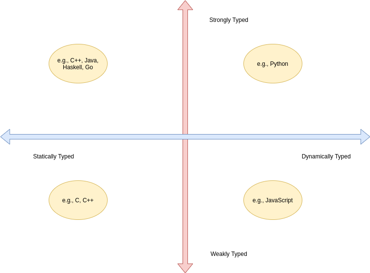
In today’s lecture we talked about types (again!). In particular, we talked about the two independent axis of types for a programming language: whether a PL is statically or dynamically typed and whether it is strongly or weakly typed. In other words, the time of the binding of type/variable in a language is independent of that language’s ability to detect type errors.

A statically typed language is one where the type/variable binding is done before the code is run and does not change throughout program execution.
A dynamically typed language is one where the type/variable binding is done at runtime and/or may change throughout program execution.

A strongly typed language is one where type errors are always detected (either at before or during program execution)
A weakly typed language is one that is, well, not strongly typed.

In order to have a completely a satisfying definition of strongly typed language, we defined type error as any error that occurs when an operation is attempted on a type for which it is not well defined. In Python, "3" + 5 results in a TypeError: can only concatenate str (not "int") to str. In this example, the operation is + and the types are str and int.

Certain strongly typed languages appear to be weakly typed because of coercions. A coercion occurs when the language implicitly converts a variable of one type to another. C++ allows the programmer to define operations that will convert the type of a variable from, say, type a to type b. If the compiler sees an expression using a variable of type b where only a variable of type a is valid, then it will invoke that conversion operation automatically. While this adds to the language’s flexibility, the conversion behavior may hide the fact that a type error exists and, ultimately, make code more difficult to debug. Note that coercions are done implicitly – a change between types done at the explicit request of the programmer is know as a (type)cast.

Finally, before digging in to actual types, we defined type system: A type system is the set of types supported by a language and the rules for their usage.

Aggregate Data Types

Aggregate data types are data types composed of one or more basic, or primitive, data types. Do not ask me to write a specific definition for primitive data type – it will only get us into a circular mess :-)

Array

An array is a homogeneous (i.e., all its elements must be of the same type) aggregate data type in which an individual element is accessed by its position (i.e., index) in the aggregate. There are myriad design decisions associated with a language’s implementation of arrays (the type of the index, whether their size must be fixed or whether it can be dynamic, etc.) One of those design decisions is the way that a language lays out a two dimensional array in memory. There are two options: row-major order and column-major order. For a second, forget the concept of rows and columns altogether and consider that you access two dimensional arrays by letters and numbers. See the following diagram:

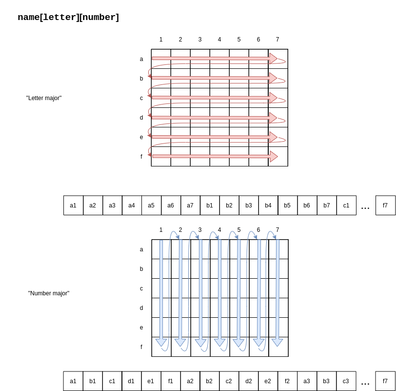The memory of actual computers is linear. Therefore, two dimensional arrays must be flattened. In “letter major” order, the slices of the array identified by letters are stored in memory one after the other. In “number major” order, the slices of the array identified by numbers are stored in memory one after another. Notice that, in “letter major” order, the numbers “change fastest” and that, in “number major” order, the letters “change fastest”.

Substitute “row” for “letter” and “column” for “number” and, voila, you understand!! The C programming language stores arrays in row-major order; Fortran stores arrays in column-major order.

Keep in mind that this description is only one way (or many) to store two dimensional arrays. There are (Links to an external site.) others (Links to an external site.).

Associative Arrays, Records, Tuples, Lists, Unions, Algebraic Data Types, Pattern Matching, List Comprehensions, and Equivalence

All that, and more, in Episode 2 of PL After Dark!

Note: In this video, I said that Python’s Lists function as arrays and that Python does not have true arrays. Your book implies as much in the section on Lists. However, I went back to check, and it does appear that there is a standard module in Python that provides arrays, in certain cases. Take a look at the documentation here: python arrays . The commonly used NumPy package also provides an array type: numpy arrays . While the language, per se, does not define an array type, the presence of the modules (particularly the former) is important to note. Sorry for the confusion!

9/10/2021

In today’s edition of the Daily PL we will recap our discussion from today that covered expressions, order of evaluation, short-circuit evaluation and referential transparency.

Expressions

An expression is the means of specifying computations in a programming language. Informally, it is anything that yields a value. For example,

5 is an expression (value 5)
5 + 2 is an expression (value 7)
Assuming fun is a function that returns a value, fun() is an expression (value is the return value)
Assuming f is a variable, f is an expression (the value is the value of the variable)

Certain languages allow more exotic statements to be expressions. For example, in C/C++, the = operator yields a value (the value of the expression on the right operand). It is this choice by the language designer that allows a C/C++ programmer to write

int a, b, c, d;
a = b = c = d = 5;

to initialize all four variables to 5.

When we discuss functional programming languages, we will see how many more things are expressions that programmers typically think are simply statements.

Order of Evaluation

Programmers learn the associativity and precedence of operations in their languages. That knowledge enables them to mentally calculate the value of statements like 5 + 4 * 3 / 2.

What programmers often forget to learn about their language, is the order of evaluation of operands. Take several of those constants from the previous expression and replace them with variables and function calls:

5 + a() * c / b()

The questions abound:

Is a() executed before the value of variable c is retrieved?
Is b() executed before c()?
Is b() executed at all?

In a language with functional side effects, the answer to these questions matter. Why? Consider that a could have a side effect that changes c. If the value of c is retrieved before the execution of a() then the expression will evaluate to a certain value and if the value of c is retrieved after execution of a() then the expression will evaluate to a different value.

Certain languages define the order of evaluation of operands (Python, Java) and others do not (C/C++). There are reasons why defining the order is a good thing:

The programmer can depend on that order and benefit from the consistency
The program’s readability is improved.
The program’s reliability is improved.

But there is at least one really good reason for not defining that order: optimizations. If the compiler/interpreter can move around the order of evaluation of those operands, it may be able to find a way to generate faster code!

Short-circuit Evaluation

Languages with short-circuit evaluation take these potential optimizations one step further. For a boolean expression, the compiler will stop evaluating the expression as soon as the result is fixed. For instance, in a() && b(), if a() is false, then the entire statement will always be false, no matter the value of b(). In this case, the compiler/interpreter will simply not execute b(). On the other hand, in a() || b() if a() is true, then the entire statement will always be true, no matter the value of b(). In this case, the compiler/interpreter will simply not execute b().

A programmer’s reliance on this type of behavior in a programming language is very common. For instance, this is a common idiom in C/C++:

int *variable = nullptr;

...

if (variable != nullptr && *variable > 5) {
  ...
}

In this code, the programmer is checking to see whether there is memory allocated to variable before they attempt to read that memory. This is defensive programming thanks to short-circuit evaluation.

Referential Transparency

Most of these issues would not be a problem if programmer’s wrote functions that did not have side effects (remember that those are called pure functions). There are languages that will not allow side effects and those languages support referential transparency: A function has referential transparency if its value (its output) depends only on the value of its parameter(s). In other words, if given the same inputs, a referentially transparent function always gives the same output.

Put It All Together

Try you hand at the practice quiz Expressions, precedence, associativity and coercions to check your understanding of the material we covered in class on Friday and the material from your assigned reading! For the why, check out relational.cpp .

9/13/2021

In today’s edition of the Daily PL we will recap our discussion from today that covered subprograms, polymorphism and coroutines!

Subprograms

A subprogram is a type of abstraction. It is process abstraction where the how of a process is hidden from the user who concerns themselves only with the what. A subprogram provides process abstraction by naming a collection of statements that define parameterized computations. Again, the collection of statements determines how the process is implemented. Subprogram parameters give the user the ability to control the way that the process executes. There are three types of subprograms:

Procedure: A subprogram that does not return a value.
Function: A subprogram that does return a value.
Method: A subprogram that operates with an implicit association to an object; a method may or may not return a value.

Pay close attention to the book’s explanation and definitions of terms like parameter, parameter profile, argument, protocol, definition, and declaration.

Subprograms are characterized by three facts:

A subprogram has only one entry point
Only one subprogram is active at any time
Program execution returns to the caller upon completion

Polymorphism

Polymorphism allows subprograms to take different types of parameters on different invocations. There are two types of polymorphism:

ad-hoc polymorphism: A type of polymorphism where the semantics of the function may change depending on the parameter types.
parametric polymorphism: A type of polymorphism where subprograms take an implicit/explicit type parameter used to define the types of their subprogram’s parameters; no matter the value of the type parameter, in parametric polymorphism the subprogram’s semantics are always the same.

Ad-hoc polymorphism is sometimes call function overloading (C++). Subprograms that participate in ad-hoc polymorphism share the same name but must have different protocols. If the subprograms’ protocols and names were the same, how would the compiler/interpreter choose which one to invoke? Although a subprogram’s protocol includes its return type, not all languages allow ad-hoc polymorphism to depend on the return type (e.g., C++). See the various definitions of add in the C++ code here: subprograms.cpp . Note how they all have different protocols. Further, note that not all the versions of the function add perform an actual addition! That’s the point of ad-hoc polymorphism – the programmer can change the meaning of a function.

Functions that are parametrically polymorphic are sometimes called function templates (C++) or generics (Java, soon to be in Go, Rust). A parametrically polymorphic function is like the blueprint for a house with a variable number of floors. A home buyer may want a home with three stories – the architect takes their variably floored house blueprint and “stamps out” a version with three floors. Some “new” languages call this process monomorphization (Links to an external site.). See the definition of minimum in the C++ code here: subprograms.cpp . Note how there is only one definition of the function. The associated type parameter is T. The compiler will “stamp out” copies of minimum for different types when it is invoked. For example, if the programmer writes


auto m = minimum(5, 4);

then the compiler will generate

int minimum(int a, int b) {

 return a < b ? a : b;
}

behind the scenes.

Coroutines

Just when you thought that you were getting the hang of subprograms, a new kid steps on the block: coroutines. Sebesta defines coroutines as a subprogram that cooperates with a caller. The first time that a programmer uses a coroutine, they call it at which point program execution is transferred to the statements of the coroutine. The coroutine executes until it yields control. The coroutine may yield control back to its caller or to another coroutine. When the coroutine yields control, it does not cease to exist – it simply goes dormant. When the coroutine is again invoked – resumed – the coroutine begins executing where it previously yielded. In other words, coroutines have

multiple entry points
full control over execution until they yield
the property that only one is active at a time (although many may be dormant)

Coroutines could be used to write a card game. Each player is a coroutine that knows about the player to their left (that is, a coroutine). The PlayerA coroutine performs their actions (perhaps drawing a card from the deck, etc) and checks to see if they won. If they did not win, then the PlayerA coroutine yields to the PlayerB coroutine who performs the same set of actions. This process continues until a player no longer has someone to their left. At that point, everything unwinds back to the point where PlayerA was last resumed – the signal that a round is complete. The process continues by resuming PlayerA to start another round of the game. Because each player is a coroutine, it never ceased to exist and, therefore, retains information about previous draws from the deck. When a player finally wins, the process completes. To see this in code, check out cardgame.py .

9/20/2021

This is an issue of the Daily PL that you are going to want to make sure that you keep safe – definitely worth framing and passing on to your children! You will want to make sure you remember where you were when you first learned about …

Formal Program Semantics

Although we have not yet learned about it (we will, don’t worry!), there is a robust set of theory around the way that PL designers describe the syntax of their language. You can use regular expressions, context-free grammars, parsers (recursive-descent, etc) and other techniques for defining what is a valid program.

On the other hand, there is less of a consensus about how a program language designer formally describes the semantics of programs written in their language. The codification of the semantics of a program written in a particular is known as formal program semantics. In other words, formal program semantics are a precise mathematical description of the semantics of an executing program. Sebesta uses the term dynamic semantics which is defines as the “meaning[] of the expressions, statements and program units of a programming language.”

The goal of defining formal program semantics is to understand and reason about the behavior of programs. There are many, many reasons why PL designers want a formal semantics of their language. However, there are two really important reasons: With formal semantics it is possible to prove that

two programs calculate the same result (in other words, that two programs are equivalent), and
a program calculates the correct result.

The alternative to formal program semantics are standards promulgated by committees that use natural language to define the meaning of program elements. Here is an example of a page from the standard for the C programming language:

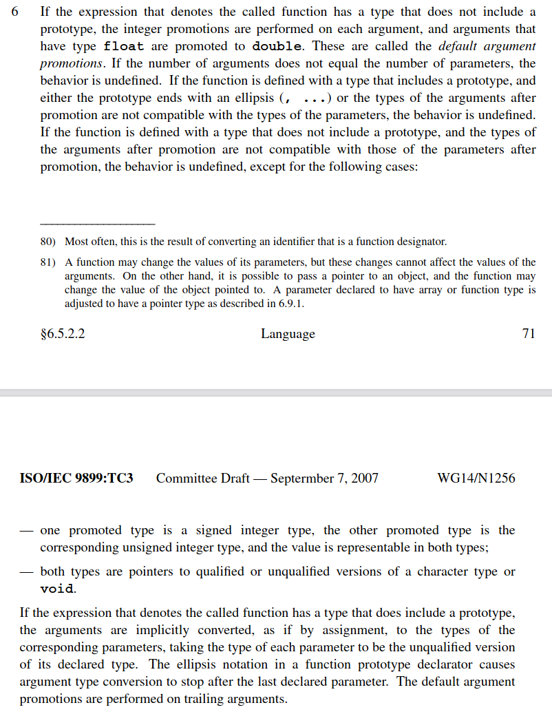
If you are interested, you can find the C++ language standard , the Java language standard , the C language standard , the Go language standard and the Python language standard all online.

Testing vs Proving

There is absolutely a benefit to testing software. No doubt about it. However, testing that a piece of software behaves a certain way does not prove that it operates a certain way.

“Program testing can be used to show the presence of bugs, but never to show their absence!” - Edsger Dijkstra

There is an entire field of computer science known as formal methods whose goal is to understand how to write software that is provably correct. There are systems available for writing programs about which things can be proven. There is PVS, Coq ,Isabelle , and TLA+ , to name a few. PVS is used by NASA to write its mission-critical software and even it makes an appearance in the movie The Martian .

Three Types of Formal Semantics

There are three common types of formal semantics. It is important that you know the names of these systems, but we will only focus on one in this course!

Operational Semantics: The meaning of a program is defined by how the program executes on an idealized virtual machine.
Denotational Semantics: Program units “denote” mathematical functions and those functions transform the mathematically defined state of the program.
Axiomatic Semantics: The meaning of the program is based on proof rules for each programming unit with an emphasis on proving the correctness of a program.

We will focus on operational semantics only!

Operational Semantics

Program State

We have referred to the state of the program throughout this course. We have talked about how statements in imperative languages can have side effects that affect the value of the state and we have talked about how the assignment statement’s raison d’etre is to change a program’s state. For operational semantics, we have to very precisely define a program’s state.

At all times, a program has a state. A state is just a function whose domain is the set of defined program variables and whose range is V * T where V is the set of all valid variable values (e.g., 5, 6.0, True, “Hello”, etc) and T is the set of all valid variable types (e.g., Integer, Floating Point, Boolean, String, etc). In other words, you can ask a state about a particular variable and, if it is defined, the function will return the variable’s current value and its type.

It is important to note that PL researchers have math envy. They are not mathematicians but they like to use Greek symbols. So, here we go:

\begin{equation*} \sigma(x) = (v, \tau) \end{equation*}

The state function is denoted with the σ . τ always represents some arbitrary variable type. Generally, v represents a value. So, you can read the definition above as “Variable x has value v and type τ in state σ.”

Program Configuration

Between execution steps (a term that we will define shortly), a program is always in a particular configuration:

\begin{equation*} <e, \sigma> \end{equation*}

This means that the program in state σ

is about to evaluate expression e.

Program Steps

A program step is an atomic (indivisible) change from one program configuration to another. Operational semantics defines steps using rules. The general form of a rule is

\begin{equation*} \frac{premises}{conclusion} \end{equation*}

The conclusion is generally written like <e, σ> ⟶ (v, τ, σ). This statement means that, when the premises hold, the rule evaluates to a value (v), type (τ) and (possibly modified) state (σ’) after a single step of execution of a program in configuration <e, σ>. Note that rules do not yield configurations. All this will make sense when we see an example.

Example 1: Defining the semantics of variable access.

In STIMPL, the expression to access a variable, say i, is written like Variable(“i”). Our operational semantic rule for evaluating such an access should “read” something like: When the program is about to execute an expression to access variable i in a state σ, the value of the expression will be the triple of i’s value, i’s type and the unchanged state σ." In other words, the evaluation of the next step of a program that is about to access a value is the value and type of the variable being accessed and the program’s state is unchanged.

Let’s write that formally!

\begin{equation*} \(\frac{\sigma(x) \rightarrow (v, \tau)} {<\text{Variable}(x), \sigma > \rightarrow (v, \tau, \sigma)}\) \end{equation*}

State Update

How do we write down that the state is being changed? Why would we want to change the state? Let’s answer the second question first: we want to change the state when, for example, there is an assignment statement. If σ (“i”) = (4, Integer) and then the program evaluated an expression like Assign(Variable(“i”), IntLiteral(2)), we don’t want the σ

function to return (4, Integer) any more! We want it to return (2, Integer). We can define that mathematically like:

\begin{equation*} \sigma[(v,\tau)/x](y)= \begin{cases} & \sigma(y) \quad y \ne x \\ &(v,\tau) \quad y=x \end{cases} \end{equation*}

This means that if you are querying the updated state for the variable that was just reassigned (x), then return its new value and type (m and τ ). Otherwise, just return the value that you would get from accessing the existing σ

Example 2: Defining the semantics of variable assignment (for a variable that already exists).

In STIMPL, the expression to overwrite the value of an existing variable, say i, with, say, an integer literal 5 is written like Assign(Variable("i"), IntLiteral(5)). Our operational semantic rule for evaluating such an assignment should “read” something like: When the program is about to execute an expression to assign variable i to the integer literal 5 in a state σ and the type of the variable i in state σ is Integer, the value of the expression will be the triple of 5, Integer and the changed state σ’ which is exactly the same as state σ

except where (5, Integer) replaced i’s earlier contents." That’s such a mouthful! But, I think we got it. Let’s replace some of those literals with symbols for abstraction purposes and then write it down!

\begin{equation*} \frac{<e, \sigma> \longrightarrow (v, \tau, \sigma’), \sigma(x) \longrightarrow (*,, \tau)} {<\text{Assign(Variable)}(x, e), \sigma > \longrightarrow (v, \tau, \sigma’ [(v, \tau)/x])} \end{equation*}

Let’s look at it step-by-step:

\begin{equation*} <Assign(Variable(x),e),\sigma> \end{equation*}

is the configuration and means that we are about to execute an expression that will assign value of expression e to variable x. But what is the value of expression e? The premise

\begin{equation} <e,\sigma>⟶(v,\tau, \sigma′) \end{equation}

tells us that the value and type of e when evaluated in state σ is v, and τ. Moreover, the premise tells us that the state may have changed during evaluation of expression e and that subsequent evaluation should use a new state, σ

‘. Our mouthful above had another important caveat: the type of the value to be assigned to variable x must match the type of the value already stored in variable x. The second premise

\begin{equation*} \sigma′(x)\longrightarrow(*, \tau) \end{equation*}

tells us that the types match – see how the τs are the same in the two premises? (We use the * to indicate that we don’t care what that value is!)

Now we can just put together everything we have and say that the expression assigning the value of expression e to variable x evaluates to

\begin{equation*} (v,\tau,\sigma′[(v,\tau)/x]) \end{equation*}

That’s Great, But Show Me Code!

Well, Will, that’s fine and good and all that stuff. But, how do I use this when I am implementing STIMPL? I’ll show you! Remember the operational semantics for variable access:

\begin{equation*} \(\frac{\sigma(x) \rightarrow (v, \tau)} {<\text{Variable}(x), \sigma > \rightarrow (v, \tau, \sigma)}\) \end{equation*}

Compare that with the code for it’s implementation in the STIMPL skeleton that you are provided for Assignment 1:

def evaluate(expression, state):
...

    case Variable(variable_name=variable_name):
      value = state.get_value(variable_name)
      if value == None:
        raise InterpSyntaxError(f"Cannot read from {variable_name} before assignment.")
      return (*value, state)

At this point in the code we are in a function named evaluate whose first parameter is the next expression to evaluate and whose second parameter is a state. Does that sound familiar? That’s because it’s the same as a configuration! We use pattern matching to select the code to execute. The pattern is based on the structure of expression and we match in the code above when expression is a variable access. Refer to Pattern Matching in Python for the exact form of the syntax. The state variable is an instance of the State object that provides a method called get_value (see Assignment 1: Implementing STIMPL for more information about that function) that returns a tuple of (v, τ) In other words, get_value works the same as σ. So,

value = state.get_value(variable_name)

is a means of implementing the premise of the operational semantics.

      return (*value, state)

yields the final result! Pretty cool, right?

Let’s do the same analysis for assignment:

\(\frac{<e,\sigma>\longrightarrow(v,\tau,\sigma′),\sigma′(x)\longrightarrow(*,\tau)}{<Assign(Variable(x),e),σ>\longrightarrow(v,\tau,σ′[(v,\tau)/x])}\)

And here’s the implementation:

def evaluate(expression, state):
...

   case Assign(variable=variable, value=value):

      value_result, value_type, new_state = evaluate(value, state)

      variable_from_state = new_state.get_value(variable.variable_name)
      _, variable_type = variable_from_state if variable_from_state else (None, None)

      if value_type != variable_type and variable_type != None:
        raise InterpTypeError(f"""Mismatched types for Assignment:
            Cannot assign {value_type} to {variable_type}""")

      new_state = new_state.set_value(variable.variable_name, value_result, value_type)
      return (value_result, value_type, new_state)

First, look at

      value_result, value_type, new_state = evaluate(value, state)

which is how we are able to find the values needed to satisfy the left-hand premise. value_result is v, value_type is τ and new_state is σ’.

      variable_from_state = new_state.get_value(variable.variable_name)

is how we are able to find the values needed to satisfy the right-hand premise. Notice that we are using new_state (σ’) to get variable.variable_name (x). There is some trickiness in_, variable_type = variable_from_state if variable_from_state else (None, None) to set things up in case we are doing the first assignment to the variable (which sets its type), so ignore that for now! Remember that in our premises we guaranteed that the type of the variable in state σ’ matches the type of the expression:

      if value_type != variable_type and variable_type != None:
        raise InterpTypeError(f"""Mismatched types for Assignment:
            Cannot assign {value_type} to {variable_type}""")

performs that check!

      new_state = new_state.set_value(variable.variable_name, value_result, value_type)

generates a new, new state (σ′[(v,τ)/x]) and


      return (value_result, value_type, new_state)

yields the final result!

9/22/2021

Like other popular newspapers that do in-depth analysis of popular topics (Links to an external site.), this edition of the Daily PL is part 2/2 of an investigative report on …

Formal Program Semantics

In our previous class, we discussed the operational semantics of variable access and variable assignment. In this class we explored the operational semantics of the addition operator and the if/then statement.

A Quick Review of Concepts

Here is the formal definition of the state function:

\begin{equation*} \(\sigma(x) = (v, \tau)\) \end{equation*}

Between execution steps, a program is always in a particular configuration:

\begin{equation*} <e, \sigma> \end{equation*}

This notation means that the program in state σ is about to evaluate expression e.

A program step is an atomic (indivisible) change from one program configuration to another. Operational semantics defines steps using rules. The general form of a rule is

\begin{equation*} \frac{premises}{conclusion} \end{equation*}

The conclusion is generally written like <e, σ> ⟶ (v, τ, σ) which means that when the premises hold, the expression e evaluated in state σ evaluates to a value (v), type (τ) and (possibly modified) state (σ’) after a single step of execution.

Defining the Semantics of the Addition Expression

In STIMPL, the expression to “add” two values n1 and n2 is written like Add(n1, n2). By the rules of the STIMPL language, for an addition to be possible, n1 and n2 must

have the same type and
have Integer, Floating Point or String type.

Because every unit in STIMPL has a value, we will define the operational semantics using two arbitrary expressions, e1 and e2. The program configuration to which we are giving semantics is

\begin{equation*} <Add(e_1),e_2),\sigma> \end{equation*}

Because our addition operator applies when its operands are three different types, we technically need three different rules for its evaluation. Let’s start with the operational semantics for add when its operands are of type Integer:

\begin{equation*} \frac{<e_1,\sigma>⟶(v_1,Integer,\sigma),<e_2,\sigma>⟶(v_2,Integer,\sigma \prime)}{<Add(e1,e2),σ>⟶(v1+v2,Integer,\sigma\prime)} \end{equation*}

Let’s look at the premises. First, there is

\begin{equation*} <e_1,\sigma>⟶(v1,Integer,\sigma \prime) \end{equation*}

which means that, when evaluated in state σ, expression e1 has the value v1 and type Integer and may modify the state (to σ’). Notice that we are not using τ for the resulting type of the evaluation? Why? Because using τ indicates that this rule applies when the evaluation of e1 in state σ evaluates to any type (which we “assign” to τ in case we want to use it again in a later premise). Instead, we are explicitly writing Integer which indicates that this rule only defines the operational semantics for Add(e1, e2) in state σ when the expression e1 evaluates to a value of type Integer in state σ

As for the second premise

\begin{equation*} <e_2,\sigma \prime>⟶(v_2,Integer,\sigma\prime \prime) \end{equation*}

we see something very similar. Again, our premise prescribes that, when evaluated in state σ’ (note the ’ there), e2’s type is an Integer. It is for this reason that we can be satisfied that this rule only applies when the types of the Add’s operands match and are integers! We “thread through” the (possibly) modified σ’ when evaluating e2 to enforce the STIMPL language’s definition that operands are evaluated strictly left-to-right.

As for the conclusion,

\begin{equation*} (v_1+v_2,Integer,\sigma \prime \prime) \end{equation*}

shows the value of this expression. We will assume here that + works as expected for two integers. Because the operands are integers, we can definitively write that the type of the addition will be an integer, too. We use σ’’ as the resulting state because it’s possible that evaluation of the expressions of both e1 and e2 caused side effects.

The rule that we defined covers only the operational semantics for addition of two integers. The other cases (for floating-point and string types) are almost copy/paste.

Now, how does that translate to an actual implementation?


def evaluate(expression, state):
  match expression:
  ...

  case Add(left=left, right=right):
      result = 0
      left_result, left_type, new_state = evaluate(left, state)
      right_result, right_type, new_state = evaluate(right, new_state)

      if left_type != right_type:
        raise InterpTypeError(f"""Mismatched types for Add:
            Cannot add {left_type} to {right_type}""")

      match left_type:
        case Integer() | String() | FloatingPoint():
          result = left_result + right_result
        case _:
          raise InterpTypeError(f"""Cannot add {left_type}s""")

      return (result, left_type, new_state)

In this snippet, the local variables left and right are the equivalent of e1 and e2, respectively, in the operational semantics. After initializing a variable to store the result, the evaluation of the premises is accomplished. new_state matches σ’’ after being assigned and reassigned in those two evaluations. Next, the code checks to make sure that the types of the operands matches. Finally, if the types of the operands is an integer, then the result is just a traditional addition (+ in Python).

You can see the implementation for the other types mixed in this code as well. Convince yourself that the code above handles all the different cases where an Add is valid in STIMPL.

Defining the Semantics of the If/Then/Else Expression

In STIMPL, we write an If/Then/Else expression like If(c, t, f) where c is any boolean-typed expression, t is the expression to evaluate if the value of c is true and f is the expression to evaluate if the value of c is false. The value/type/updated state of the entire expression is the value/type/updated state that results from evaluating t when c is true and the value/type/updated state that results from evaluating f when c is false. This means that we are required to write two different rules to completely define the operational semantics of the If/Then/Else expression: one for the case where c is true and the other for the case when c is false. Sounds like the template that we used for the Add expression, doesn’t it? Because the two cases are almost the same, we will only go through writing the rule for when the condition is true:

\begin{equation*} \frac{<c,\sigma>\longrightarrow(True,Boolean,\sigma \prime),<t,\sigma \prime>\longrightarrow(v,\tau,\sigma\prime \prime)}{<If(c,t,f),σ>⟶(v,\tau, \sigma \prime \prime)} \end{equation*}

As in the premises for the operational semantics of the Add operator, the first premise in the operational semantics above uses literals to guarantee that the rule only applies in certain cases:

\begin{equation*} <c,\sigma \prime>\longrightarrow(True,Boolean,\sigma\prime \prime) \end{equation*}

means that the rule only applies when c, evaluated in state σ, has a value of True and a boolean type. We use the second premise

\begin{equation*} <t,\sigma\prime>⟶(v,\tau,\sigma \prime \prime) \end{equation*}

to “get” some values that we will use in the conclusion. v and τ are the value and the type, respectively, of t when it is evaluated in state σ’. Note that we evaluate t in state σ’ because the evaluation of the condition statement may have modified state σ and we want to thread that through. Evaluation of t in state σ’ may modify σ’, generating σ’’. The combination of these premises are combined to define that the entire expression evaluates to

\begin{equation*} (v,\tau,\sigma\prime \prime) \end{equation*}

Again, the pattern is the same for writing the operational semantics when the condition is false.

Let’s look at how this translates into actual working code:

def evaluate(expression, state):
  match expression:
  ...

    case If(condition=condition, true=true, false=false):
      condition_value, condition_type, new_state = evaluate(condition, state)

      if not isinstance(condition_type, Boolean):
        raise InterpTypeError("Cannot branch on non-boolean value!")

      result_value = None
      result_type = None

      if condition_value:
        result_value, result_type, new_state = evaluate(true, new_state)
      else:
        result_value, result_type, new_state = evaluate(false, new_state)

      return (result_value, result_type, new_state)

The local variables condition, true and false match c, t and f, respectively from the rule in the operational semantics. The first step in the implementation is to determine the value/type/updated state when c is evaluated in state σ. Immediately after doing that, the code checks to make sure that the condition statement has boolean type. Remember how our rule only applies when this is the case? Next, depending on whether the condition evaluated to true or false, the appropriate next expression is evaluated in the σ’ state (new_state). It is the result of that evaluation that is the ultimate value of the expression and what is returned.

9/24/2021

As we conclude the penultimate week of September, we are turning the page from imperative programming and beginning our work on object-oriented programming!

The Definitions of Object-Oriented Programming

We started off by attempting to describe object-oriented programming using two different definitions:

A language with support for abstraction of abstract data types (ADTs). (from Sebesta)
A language with support for objects, containers of data (attributes, properties, fields, etc.) and code (methods). (from Wikipedia (Links to an external site.))

As graduates of CS1021C and CS1080C, the second definition is probably not surprising. The first definition, however, leaves something to be desired. Using Definition (1) means that we have to a) know the definition of abstraction and abstract data types and b) know what it means to apply abstraction to ADTs.

Abstraction (Reprise)

There are two fundamental types of abstractions in programming: process and data. We have talked about the former but the latter is new. When we talked previously about process abstractions, we did attempt to define the term abstraction but it was not satisfying.

Sebesta formally defines abstraction as the view or representation of an entity that includes only the most significant attributes. This definition seems to align with our notion of abstraction especially the way we use the term in phrases like “abstract away the details.” It didn’t feel like a good definition to me until I thought of it this way:

Consider that you and I are both humans. As humans, we are both carbon based and have to breath to survive. But, we may not have the same color hair. I can say that I have red hair and you have blue hair to point out the significant attributes that distinguish us. I need not say that we are both carbon based and have to breath to survive because we are both human and we have abstracted those facts into our common humanity.

We returned to this point at the end of class when we described how inheritance is the mechanism of object-oriented programming that provides abstraction over ADTs. Abstract Data Types (ADTs)

Next, we talked about the second form of abstraction available to programmers: data abstraction. As functions, procedures and methods are the syntactic and semantic means of abstracting processes in programming languages, ADTs are the syntactic and semantic means of abstracting data in programming languages. ADTs combine (encapsulate) data (usually called the ADT’s attributes, properties, etc) and operations that operate on that data (usually called the ADT’s methods) into a single entity.

We discussed that hiding is a significant advantage of ADTs. ADTs hide the data being represented and allow that data’s manipulation only through pre-defined methods, the ADT’s interface. The interface typically gives the ADT’s user the ability to manipulate/access the data internal to the type and perform other semantically meaningful operations (e.g., sorting a list).

We brainstormed some common ADTs:

Stack
Queue
List
Array
Dictionary
Graph
Tree

These are are so-called user-defined ADTs because they are defined by the user of a programming language and composed of primitive data types.

Next, we tackled the question of whether primitives are a type of ADT. A primitive type like floating point numbers would seem to meet the definition of an abstract data type:

It’s underlying representation is hidden from the user (the programmer does not care whether FPs are represented according to IEEE754 or some other specification)
There are operations that manipulate the data (addition, subtraction, multiplation, division).

The Requirements of an Object-Oriented Programming Language

ADTs are just one of the three requirements that your textbook’s author believes are required for a language to be considered object oriented. Sebesta believes that, in addition to ADTs, an object-oriented programming language requires support for inheritance and dynamic method binding.

Inheritance

It is inheritance where OOPs provide abstraction for ADTs. Inheritance allows programmers to abstract ADTs into common classes that share common characteristics. Consider three ADTs that we identified: trees, linked lists and graphs. These three ADTs all have nodes (of some kind or another) which means that we could abstract them into a common class: node-based things. A graph would inherit from the node-based things ADT so that its implementer could concentrate on what makes it distinct – its edges, etc.

Don’t worry if that is too theoretical. It does not negate the fact that, through inheritance, we are able to implement hierarchies that can be “read” using “is a” the way that inheritance is usually defined. With inheritance, cats inherit from mammals and “a cat is a mammal”.

Subclasses inherit from ancestor classes. In Java, ancestor classes are called superclasses and subclasses are called, well, subclasses. In C++, ancestor classes are called base classes and subclasses are called derived classes. Subclasses inherit both data and methods.

Dynamic Method Binding

In an OOP, a variable that is typed as Class A can be assigned anything that is actually a Class A or subclass thereof. We have not officially covered this yet, but in OOP a subclass can redefine a method defined in its ancestor.

Assume that every mammal can make a noise. That means that every dog can make a noise just like every cat can make a noise. Those noises do not need to be the same, though. So, a cat “overrides” the mammal’s default noise and implements their own (meow). A dog does likewise (bark). A programmer can define a variable that holds a mammal and that variable can contain either a dog or a cat. When the programmer invokes the method that causes the mammal to make noise, then the appropriate method must be called depending on the actual type in the variable at the time. If the mammal held a dog, it would bark. If the mammal held a cat, it would meow.

This resolution of methods at runtime is known as dynamic method binding.

OOP Example with Inheritance and Dynamic Method Binding


abstract class Mammal {
  protected int legs = 0;
  Mammal() {
    legs = 0;
  }
  abstract void makeNoise();
}

class Dog extends Mammal {
  Dog() {
    super();
    legs = 4;
  }
  void makeNoise() {
    System.out.println("bark");
  }
}

class Cat extends Mammal {
  Cat() {
    super();
    legs = 4;
  }

  void makeNoise() {
    System.out.println("meow");
  }
}

public class MammalDemo {
  static void makeARuckus(Mammal m) {
    m.makeNoise();
  }
  public static void main(String args[]) {
    Dog fido = new Dog();
    Cat checkers = new Cat();

    makeARuckus(fido);
    makeARuckus(checkers);
  }
}

This code creates a hierarchy with Mammal at the top as the superclass of both the Dog and the Cat. In other words, Dog and Cat inherit from Mammal. The abstract keyword before class Mammal indicates that Mammal is a class that cannot be directly instantiated. We will come back to that later. The Mammal class declares that there is a method that each of its subclasses must implement – the makeNoise function. If a subclass of Mammal fails to implement that function, it will not compile. The good news is that Cat and Dog do both implement that function and define behavior in accordance with their personality!

The function makeARuckus has a parameter whose type is a Mammal. As we said above, in OOP that means that I can assign to that variable a Mammal or anything that inherits from Mammal. When we call makeARuckus with an argument whose type is Dog, the function relies of dynamic method binding to make sure that the proper makeNoise function is called – the one that barks – even though makeARuckus does not know whether m is a generic Mammal, a Dog or a Cat. It is because of dynamic method binding that the code above generates

bark
meow

as output.

9/27/2021

It’s the last week of September but the first full week of OOP. Let’s do this!

Overriding in OOP

Recall the concept of inheritance that we discussed in the last class. Besides its utility as a formalism that describes the way a language supports abstraction of ADTs (and, therefore, makes it a plausibly OO language), inheritance provides a practical benefit in software engineering. Namely, it allows developers to build hierarchies of types.

Hierarchies are composed of pairs of classes – one is the superclass and the other is the subclass. A superclass could conceivably be itself a subclass. A subclass could itself be a superclass. In terms of a family tree, we could say that the subclass is a descendant of the superclass (Note: remember that the terms superclass and subclass are not always the ones used by the languages themselves; C++ refers to them as base and derived classes, respectively).

A subclass inherits both the data and methods from its superclass(es). However, as Sebesta says, “… the features and capabilities of the [superclass] are not quite right for the new use.” Overriding methods allows the programmer to keep most of the functionality of the baseclass and customize the parts that are “not quite right.”

An overridden method is defined in a subclass and replaces the method with the same name (and usually protocol) in the parent.

The official documentation and tutorials for Java describe overriding in the language this way:“An instance method in a subclass with the same signature (name, plus the number and the type of its parameters) and return type as an instance method in the superclass overrides the superclass’s method.” The exact rules for overriding methods in Java are online at the language specification .

Let’s make it concrete with an example:


class Car {
  protected boolean electric = false;
  protected int wheels = 4;

  Car() {
  }

  boolean ignite() {
      System.out.println("Igniting a generic car's engine!");
      return true;
  }
}

class Tesla extends Car {
  Tesla() {
    super();
    electric = true;
  }

  @Override
  boolean ignite() {
    System.out.println("Igniting a Tesla's engine!");
    return true;
  }
}

class Chevrolet extends Car {
  Chevrolet() {
    super();
  }

  @Override
  boolean ignite() {
    System.out.println("Igniting a Chevrolet's engine!");
    return false;
  }
}

In this example, Car is the superclass of Tesla and Chevrolet. The Car class defines a method named ignite. That method will ignite the engine of the car – an action whose mechanics differ based on the car’s type. In other words, this is a perfect candidate for overriding. Both Tesla and Chevrolet implement a method with the same name, return value and parameters, thereby meeting Java’s requirements for overriding. In Java, the @Override is known as an annotation. Annotations are “a form of metadata [that] provide data about a program that is not part of the program itself.” Annotations in Java are attached to particular syntactic units. In this case, the @Override annotation is attached to a method and it tells the compiler that the method is overriding a method from its superclass. If the compiler does not find a method in the superclass(es) that is capable of being overridden by the method, an error is generated. This is a good check for the programmer. (Note: C++ offers similar functionality through the override specifier (Links to an external site.).)

Let’s say that the programmer actually implemented the Tesla class like this:


class Tesla extends Car {
  Tesla() {
    super();
    electric = true;
  }

  @Override
  boolean ignite(int testing) {
    super.ignite();
    System.out.println("Igniting a Tesla's engine!");
    return true;
  }
}

The ignite method implemented in Tesla does not override the ignite method from Car because it has a different set of parameters. The @Override annotation tells the compiler that the programmer thought they were overriding something. An error is generated and the programmer can make the appropriate fix. Without the @Override annotation, the code will compile but produce incorrect output when executed.

Assume that the following program exists:


public class CarDemo {
  public static void main(String args[]) {
    Car c = new Car();
    Car t = new Tesla();
    Car v = new Chevrolet();

    c.ignite();
    t.ignite();
    v.ignite();
  }
}

This code instantiates three different cars – the first is a generic Car, the second is a Tesla and the third is a Chevrolet. Look carefully and note that the type of each of the three is actually stored in a variable whose type is Car and not a more-specific type (ie, Tesla or Chevy). This is not a problem because of dynamic dispatch. At runtime, the JVM will find the proper ignite function and invoke it according to the variable’s actual type and not its static type. Because ignite is overridden by Chevy and Tesla, the output of the program above is:

Igniting a generic car's engine!
Igniting a Tesla's engine!
Igniting a Chevrolet's engine!

Most OOP languages provide the programmer the option to invoke the method they are overriding from the superclass. Java is no different. If an overriding method implementation wants to invoke the functionality of the method that it is overriding, it can do so using the super keyword.


class Tesla extends Car {
  Tesla() {
    super();
    electric = true;
  }

  @Override
  boolean ignite() {
    super.ignite();
    System.out.println("Igniting a Tesla's engine!");
    return true;
  }
}

class Chevrolet extends Car {
  Chevrolet() {
    super();
  }

  @Override
  boolean ignite() {
    super.ignite();
    System.out.println("Igniting a Chevrolet's engine!");
    return false;
  }
}

With these changes, the program now outputs:

Igniting a generic car's engine!
Igniting a generic car's engine!
Igniting a Tesla's engine!
Igniting a generic car's engine!
Igniting a Chevrolet's engine!

New material alert: What if the programmer does not want a subclass to be able to customize the behavior of a certain method? For example, no matter how you subclass Dog, it’s noise method is always going to bark – no inheriting class should change that. Java provides the final keyword to guarantee that the implementation of a method cannot be overridden by a subclass. Let’s change the code for the classes from above to look like this:


class Car {
  protected boolean electric = false;
  protected int wheels = 4;

  Car() {
  }

  void start() {
    System.out.println("Starting a car ...");
    if (this.ignite()) {
      System.out.println("Ignited the engine!");
    } else {
      System.out.println("Did NOT ignite the engine!");
    }
  }

  final boolean ignite() {
      System.out.println("Igniting a generic car's engine!");
      return true;
  }
}

class Tesla extends Car {
  Tesla() {
    super();
    electric = true;
  }

  @Override
  boolean ignite() {
    super.ignite();
    System.out.println("Igniting a Tesla's engine!");
    return true;
  }
}

class Chevrolet extends Car {
  Chevrolet() {
    super();
  }

  @Override
  boolean ignite() {
    super.ignite();
    System.out.println("Igniting a Chevrolet's engine!");
    return false;
  }
}

Notice that ignite in the Car class has a final before the return type. This makes ignite a final method : “A method can be declared final to prevent subclasses from overriding or hiding it”. (C++ has something similar – the final specifier .) Attempting to compile the code above produces this output:


CarDemo.java:30: error: ignite() in Tesla cannot override ignite() in Car
  boolean ignite() {
          ^
  overridden method is final
CarDemo.java:43: error: ignite() in Chevrolet cannot override ignite() in Car
  boolean ignite() {
          ^
  overridden method is final
2 errors

Subclass vs Subtype

In OOP there is fascinating distinction between subclasses and subtypes. All those classes that inherit from other classes are considered subclasses. However, they are not all subtypes. For a type/class S to be a subtype of type/class T, the following must hold

Assume that ϕ(t) is some provable property that is true of t, an object of type T. Then ϕ(s)

must be true as well for s, an object of type S.

This formal definition can be phrased simply in terms of behaviors: If it is possible to pass objects of type T as arguments to a function that expects objects of type S without any change in the behavior, then S is a subtype of T. In other words, a subtype behaves exactly like the “supertype”.

Barbara Liskov who pioneered the definition and study of subtypes put it this way (Links to an external site.): “If for each object o1 of type S there is an object o2 of type T such that for all programs P defined in terms of T, the behavior of P is unchanged when o1 is substituted for o2, then S is a subtype of T.”

Open Recursion

Open recursion in an OO PL is a fancy term for the combination of a) functionality that gives the programmer the ability to refer to the current object from within a method (usually through a variable named this or self) and b) dynamic dispatch. . Thanks to open recursion, some method A of class C can call some method B of the same class. But wait, there’s more! (Links to an external site.) Continuing our example, in open recursion, if method B is overriden in class D (a subclass of C), then the overriden version of the method is invoked when called from method A on an object of type D even though method A is only implemented by class C. Wild! It is far easier to see this work in real life than talk about it abstractly. So, consider our cars again:

class Car {
  protected boolean electric = false;
  protected int wheels = 4;

  Car() {
  }

  void start() {
    System.out.println("Starting a car ...");
    if (this.ignite()) {
      System.out.println("Ignited the engine!");
    } else {
      System.out.println("Did NOT ignite the engine!");
    }
  }

  boolean ignite() {
      System.out.println("Igniting a generic car's engine!");
      return true;
  }
}

class Tesla extends Car {
  Tesla() {
    super();
    electric = true;
  }

  @Override
  boolean ignite() {
    System.out.println("Igniting a Tesla's engine!");
    return true;
  }
}

class Chevrolet extends Car {
  Chevrolet() {
    super();
  }

  @Override
  boolean ignite() {
    System.out.println("Igniting a Chevrolet's engine!");
    return false;
  }
}

The start method is only implemented in the Car class. At the time that it is compiled, the Car class has no awareness of any subclasses (ie, Tesla and Chevrolet). Let’s run this code and see what happens:


public class CarDemo {
  public static void main(String args[]) {
    Car c = new Car();
    Car t = new Tesla();
    Car v = new Chevrolet();

    c.start();
    t.start();
    v.start();
  }
}

Here’s the output:

Starting a car ...
Igniting a generic car's engine!
Ignited the engine!
Starting a car ...
Igniting a Tesla's engine!
Ignited the engine!
Starting a car ...
Igniting a Chevrolet's engine!
Did NOT ignite the engine!

Wow! Even though the implementation of start is entirely within the Car class and the Car class knows nothing about the Tesla or Chevrolet subclasses, when the start method is invoked on object’s of those types, the call to this’s ignite method triggers the execution of code specific to the type of car!

How cool is that?

10/1/2021

Original is here.

We made it into October!! Spooky, spooky!

Corrections

Like in real newspapers (Links to an external site.), we are going to start including Corrections in each edition! We want to make sure that our reporters adhere to the highest standards:

The JVM will insert an implicit call to the to-be-instantiated class’ default constructor (i.e., the one with no parameters) if the the to-be-constructed (sub)class does not do so explicitly. We’ll make this clear with an example:


class Parent {
  Parent() {
    System.out.println("I am in the Parent constructor.");
  }

  Parent(int parameter) {
    System.out.println("This version of the constructor is not called.");
  }
}

class Child extends Parent {
  Child() {
    /*
     * No explicit call to super -- one is automatically
     * injected to the parent constructor with no parameters.
     */
    System.out.println("I am in the Child constructor.");
  }
}

public class DefaultConstructor {
  public static void main(String args[]) {
    Child c = new Child();
  }
}

When this program is executed, it will print

I am in the Parent constructor.
I am in the Child constructor.

The main function is instantiating an object of the type Child. We can visually inspect that there is no explicit call the super() from within the Child class’ constructor. Therefore, the JVM will insert an implicit call to super() which actually invokes Parent().

However, if we make the following change:

class Parent {
  Parent() {
    System.out.println("I am in the Parent constructor.");
  }

  Parent(int parameter) {
    System.out.println("This version of the constructor is not called.");
  }
}

class Child extends Parent {
  Child() {
    /*
     * No explicit call to super -- one is automatically
     * injected to the parent constructor with no parameters.
     */
    super(1);
    System.out.println("I am in the Child constructor.");
  }
}

public class DefaultConstructor {
  public static void main(String args[]) {
    Child c = new Child();
  }
}

Something different happens. We see that there is a call to Child’s superclass’ constructor (the one that takes a single int-typed parameter). That means that the JVM will not insert an implicit call to super() and we will get the following output:

This version of the constructor is not called. I am in the Child constructor.

The C++ standard sanctions a main function without a return statement. The standard says: “if control reaches the end of main without encountering a return statement, the effect is that of executing return 0;.”

A Different Way to OOP

So far we have talked about OOP in the context of Java. Java, and languages like it, are called Class-based OOP languages. In a Class-based OOP, classes and objects exist in different worlds. Classes are used to define/declare

the attributes and methods of an encapsulation, and
the relationships between them.

From these classes, objects are instantiated that contain those attributes and methods and respect the defined/declared hierarchy. We can see this in the example given above: The classes Parent and Child define (no) attributes and (no) methods and define the relationship between them. In main(), a Child is instantiated and stored in the variable c. c is an object of type Child that contains all the data associated with a Child and a Parent and can perform all the actions of a Child and a Parent.

Nothing about Class-based OOP should be different than what you’ve learned in the past as you’ve worked with C++. There are several problems with Class-based OOP.

The supported attributes and method of each class must be determined before the application is developed (once the code is compiled and the system is running, an object cannot add, remove or modify its own methods or attributes);
The inheritance hierarchy between classes must be determined before the application is developed (once the code is compiled, changing the relationship between classes will require that the application be recompiled!).

In other words, Class-based OOP does not allow the structure of the Classes (nor their relationships) to easily evolve with the implementation of a system.

There is another way, though. It’s called Prototypal OOP. The most commonly known languages that use Prototypal OOP are JavaScript and Ruby! In Prototypal (which is a very hard word to spell!) OOP there is no distinction between Class and object – everything is an object! In a Prototypal OOP there is a base object that has no methods or data attributes and every object is able to modify itself (its attributes and methods). To build a new object, the programmer simply copies from an existing object, the new object’s so-called prototype, and customizes the copied object appropriately.

For example, assume that there is an object called Car that has one attribute (the number of wheels) and one method (start). That object can serve as the prototype car. To “instantiate” a new Car, the programmer simply copies the existing prototypical car object Car and gives it a name, say, c. The programmer can change the value of c’s number of wheels and invoke its method, start. Let’s say that the same programmer wants to create something akin to a subclass of Car. The programmer would create a new, completely fresh object (one that has no methods or attributes), name it, say, Tesla, and link the new prototype Tesla object to the existing prototype car Car object through the prototype Tesla object’s prototype link (the sequence of links that connects prototype objects to one another is called a prototype chain). If a Tesla has attributes (range, etc) or methods (self_drive) that the prototype car does not, then the programmer would install those methods on the prototype Tesla Tesla. Finally, the programmer would “declare” that the Tesla object is a prototype Tesla.

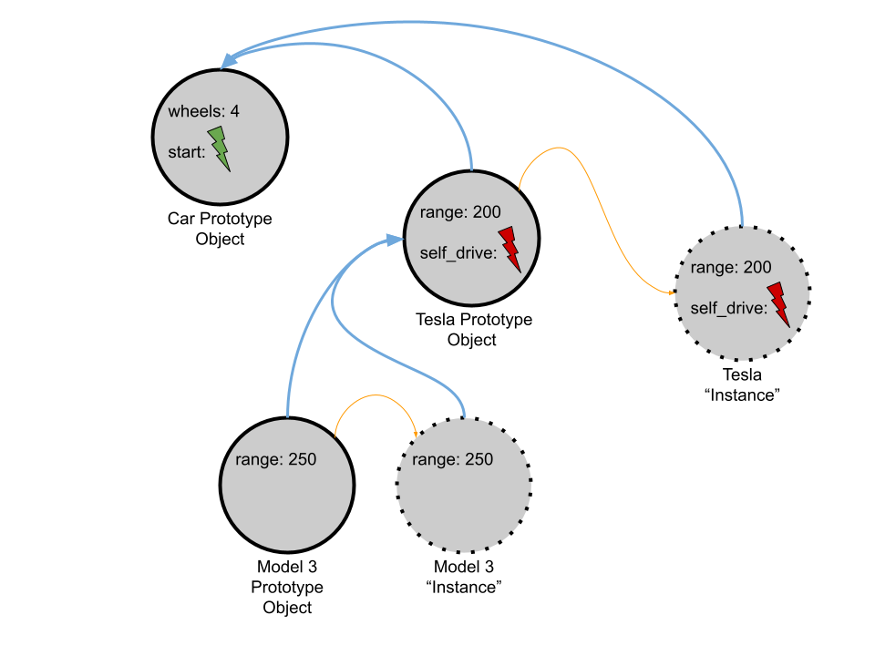
The blue arrows in the diagram above are prototype links. The orange lines indicate where a copy is made.

How does inheritance work in such a model? Well, it’s actually pretty straightforward: When a method is invoked or an attribute is read/assigned, the runtime will search the prototype chain for the first prototypical object that has such a method or attribute. Mic drop. In the diagram above, let’s follow how this would play out when the programmer calls start() on the Model 3 Instance. The Model 3 Instance does not contain a method named start. So, up we go! The Tesla Prototype Object does not contain that me either. All the way up! The Car Prototype Object, does, however, so that method is executed!

What would it look like to override a function? Again, relatively straightforward. If a Tesla performs different behavior than a normal Car when it starts, the programmer creating the Tesla Prototype Object would just add a method to that object with the name start. Then, when the prototype chain is traversed by the runtime looking for the method, it will stop at the start method defined in the Tesla Prototype Object instead of continuing on to the start method in the Car Prototype Object. (The same is true of attributes!)

There is (at least) one really powerful feature of this model. Keep in mind that the prototype objects are real things that can be manipulated at runtime (unlike classes which do not really exist after compilation) and prototype objects are linked together to achieve a type of inheritance. With reference to the diagram above, say the programmer changes the definition of the start method on the Car Prototype Object. With only that change, any object whose prototype chain includes the Car Prototype Object will immediately have that new functionality (where it is not otherwise overridden, obviously) – all without stopping the system!! How cool is that?

How scary is that? Can you imagine working on a system where certain methods you “inherit” change at runtime?

OOP or Interfaces?

Newer languages (e.g., Go, Rust, (new versions of) Java) are experimenting with new features that support one of the “killer apps” of OOP: The ability to define a function that takes a parameter of type A but that works just the same as long as it is called with an argument whose type is a subtype of A. The function doesn’t have care whether it is called with an argument whose type is A or some subtype of A because the language’s OOP semantics guarantee that anything the programmer can do with an object of type A, the programmer can do with and object of subtype of A.

Unfortunately, using OOP to accomplish such a feat may be like killing a fly with a bazooka (or a laptop, like Alex killed that wasp today).

Instead, modern languages are using a slimmer mechanism known as an interface or a trait. An interface just defines a list of methods that an implementer of that interface must support. Let’s see some real Go code that does this – it’ll clear things up:


type Readable interface {
  Read()
}

This snippet defines an interface with one function (Read) that takes no parameters and returns no value. That interface is named Readable. Simple.


type Book struct {
  title string
}

This snippet defines a data structure called a Book – such structs are the closest that Go has to classes.


func (book Book) Read() {
  fmt.Printf("Reading the book %v\n", book.title)
}

This snippet simply says that if variable b is of type Book then the programmer can call b.Read(). Now, for the payoff:


func WhatAreYouReading(r Readable) {
  r.Read()
}

This function only accepts arguments that implement (i.e., meet the criteria specified in the definition of) the Readable interface. In other words, with this definition, the code in the body of the function can safely assume that it can can call Read on r. And, for the encore:


  book := Book{title: "Infinite Jest"}
  WhatAreYouReading(book)

This code works exactly like you’d expect. book is a valid argument to WhatAreYouReading because it implements the Read method which, implicitly, means that it implements the Readable interface. But, what’s really cool is that the programmer never had to say explicitly that Book implements the Readable interface! The compiler checks automatically. This gives the programmer the ability to generate a list of only the methods absolutely necessary for its parameters to implement to achieve the necessary ends – and nothing unnecessary. Further, it decouples the person implementing a function from the person using the function – those two parties do not have to coordinate requirements beforehand. Finally, this functionality means that a structure can implement as few or as many interfaces as its designer wants.

Dip Our Toe Into the Pool of Pointers

We only had a few minutes to start pointers, but we did make some headway. There will be more on this in the next lecture!

It is important to remember that pointers are like any other type – they have a range of valid values and a set of valid operations that you can perform on those values. What are the range of valid values for a pointer? All valid memory addresses. And what are the valid operations? Addition, subtraction, dereference and assignment.

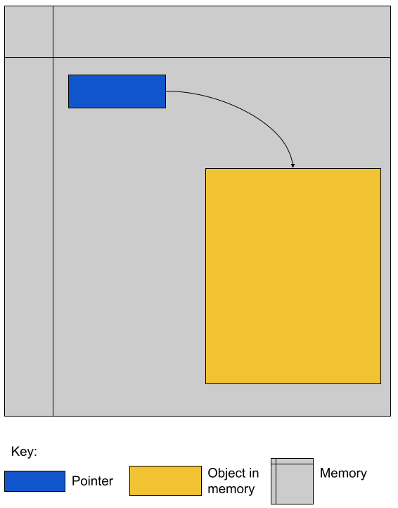
In the diagram, the gray area is the memory of the computer. The blue box is a pointer. It points to the gold area of memory. It is important to remember that pointers and their targets both exist in memory! In fact, in true Inception (Links to an external site.)style, a pointer can pointer to a pointer!

At the same time that pointers are types, they also have types. The type of a pointer includes the type of the target object. In other words, if the memory in the gold box held an object of type T, the the green box’s type would be “pointer to type T.” If the programmer dereferences the blue pointer, they will get access to the object in memory in the gold.

In an ideal scenario, it would always be the case that the type of the pointer and the type of the object at the target of the pointer are the same. However, that’s not always the case. Come to the next lecture to see what can go wrong when that simple fact fails to hold!

10/4/2021

Original is here One day closer to Candy Corn!

Corrections

When we were discussing the nature of the type of pointers, we specified that the range of valid values for a pointer are all memory addresses. In some languages this may be true. However, some other languages specify that the range of valid values for a pointer are all memory addresses and a special null value that explicitly specifies a pointer does not point to a target.

We also discussed the operations that you can perform on a pointer-type variable. What we omitted was a discussion of an operation that will fetch the address of a variable in memory. For languages that use pointers to support indirect addressing (see below), such an operation is required. In C/C++, this operation is performed using the address of (&) operator.

Pointers

We continued the discussion of pointers that we started on Friday! On Friday we discussed that pointers are just like any other type – they have valid values and defined operations that the programmer can perform on those values.

The Pros of Pointers

Though a very famous and influential computer scientist (Links to an external site.) once called his invention of null references a “billion dollar mistake” (he low balled it, I think!), the presence and power of pointers in a language is important for at least two reasons:

Without pointers, the programmer could not utilize the power of indirection.
Pointers give the programmer the power to address and manage heap-dynamic memory.

Indirection gives the programmer the power to link between different objects in memory – something that makes writing certain data structures (like trees, graphs, linked lists, etc) easier. Management of heap-dynamic memory gives the programmer the ability to allocate, manipulate and deallocate memory at runtime. Without this power, the programmer would have to know before execution the amount of memory their program will require.

The Cons of Pointers

Their use as a means of indirection and managing heap-dynamic memory are powerful, but misusing either can cause serious problems.

Possible Problems when Using Pointers for Indirection

As we said in the last lecture, as long as a pointer targets memory that contains the expected type of object, everything is a-okay. Problems arise, however, when the target of the pointer is an area in memory that does not contain an object of the expected type (including garbage) and/or the pointer targets an area of memory that is inaccessible to the program.

The former problem can arise when code in a program writes to areas of memory beyond their control (this behavior is usually an error, but is very common). It can also arise because of a use after free. As the name implies, a use-after-free error occurs when a program uses memory after it has been freed. There are two common scenarios that give rise to a use after free:
1. Scenario 1:
  1. One part of a program (part A) frees an area of memory that held a variable of type T that it no longer needs
  2. Another part of the program (part B) has a pointer to that very memory
  3. A third part of the program (part C) overwrites that “freed” area of memory with a variable of type S
  4. Part B accesses the memory assuming that it still holds a variable of Type T
2. Scenario 2:
  1. One part of a program (part A) frees an area of memory that held a variable of type T that it no longer needs
  2. Part A never nullifies the pointer it used to point to that area of memory though the pointer is now invalid because the program has released the space
  3. A second part of the program (part C) overwrites that “freed” area of memory with a variable of type S
  4. Part A incorrectly accesses the memory using the invalid pointer assuming that it still holds a variable of Type T
Scenario 2 is depicted visually in the following scenario and intimates why use-after-free errors are considered security vulnerabilities:

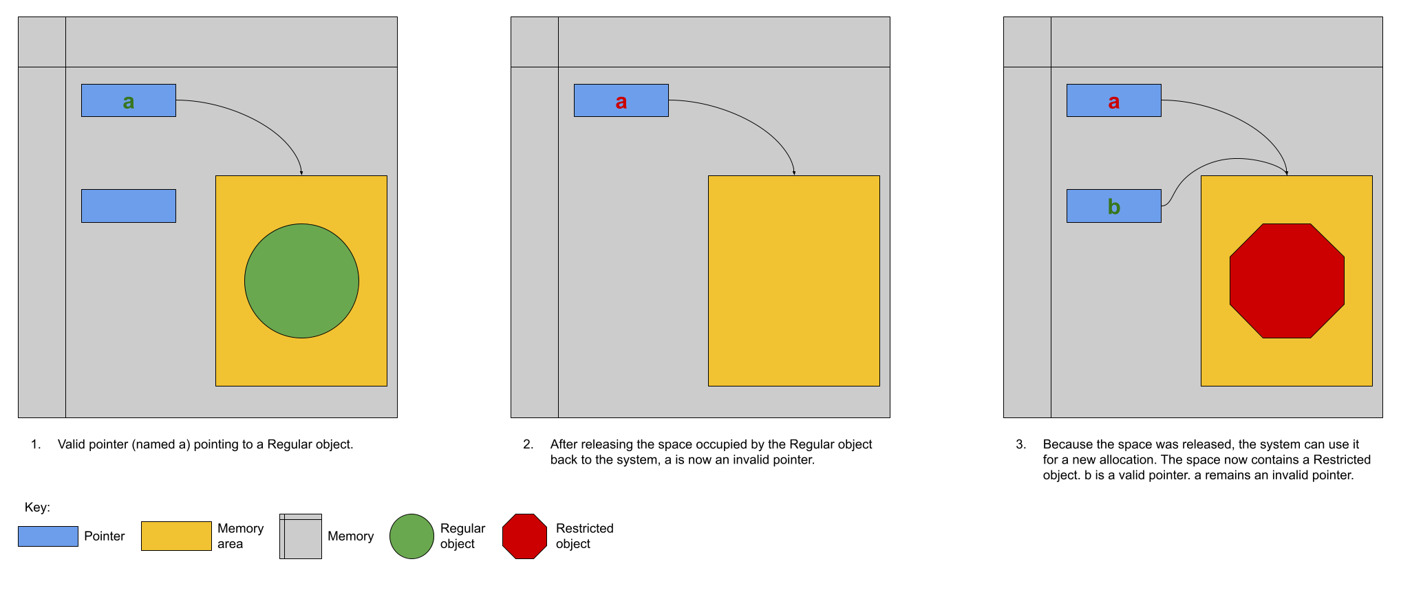
In the example shown visually above, the program’s use of the invalid pointer means that the user of the invalid pointer can now access an object that is at a higher privilege level (Restricted vs Regular) than the programmer intended. When the programmer calls a function through the invalid pointer they expect that a method on the Regular object will be called. Unfortunately, a method on the Restricted object will be called instead. Trouble!

The latter problem occurs when a pointer targets memory beyond the program’s control. This most often occurs when the program sets a variable’s address to 0 (NULL, null, nil) to indicate that it is invalid but later uses that pointer without checking its validity. For compiled languages this often results in the dreaded segmentation fault and for interpreted languages it often results in other anomalous behavior (like Java’s Null Pointer Exception (NPE)). Neither are good!

Possible Solutions

Wouldn’t it be nice if we had a way to make sure that the pointer being dereferenced is valid so we fall victim to some of the aforementioned problems? What would be the requirements of such a solution?
1. Pointers to areas of memory that have been deallocated cannot be dereferenced.
2. The type of the object at the target of a pointer always matches the programmer’s expectation.
Your author describes two potential ways of doing this. First, are tombstones. Tombstones are essentially an intermediary between a pointer and its target. When the programming language implements pointers and uses tombstones for protection, a new tombstone is allocated for each pointer the programmer generates. The programmer’s pointer targets the tombstone and the tombstone targets the pointer’s actual target. The tombstone also contains an extra bit of information: whether it is valid. When the programmer first instantiates a pointer to some target a the compiler/interpreter
1. generates a tombstone whose target is a
2. sets the valid bit of the tombstone to valid
3. points the programmer’s pointer to the tombstone.
When the programmer dereferences their pointer, the compiler/runtime will check to make sure that the target tombstone’s valid flag is set to valid before doing the actual dereference of the ultimate target. When the programmer “destroys” the pointer (by releasing the memory at its target or by some other means), the compiler/runtime will set the target tombstone’s valid flag to invalid. As a result, if the programmer later attempts to dereference the pointer after it was destroyed, the compiler/runtime will see that the tombstone’s valid flag is invalid and generate an appropriate error.

This process is depicted visually in the following diagram.

Tombstones.png

This seems like a great solution! Unfortunately, there are downsides. In order for the tombstone to provide protection for the entirety of the program’s execution, once a tombstone has been allocated it cannot be reclaimed. It must remain in place forever because it is always possible that the programmer can incorrectly reuse an invalid pointer. As soon as the tombstone is deallocated, the protection that it provides is gone. The other problem is that the use of tombstones adds an additional layer of indirection to dereference a pointer and every indirection causes memory accesses. Though memory access times are small, they are not zero – the cost of these additional memory accesses add up.

What about a solution that does not require an additional level of indirection? There is a so-called lock-and-key technique. This protection method requires that the pointer hold an additional piece of information beyond the address of the target: the key. The memory at the target of the pointer is also required to hold a key. When the system allocates memory it sets the keys of the pointer and the target to be the same value. When the programmer dereferences a pointer, the two keys are compared and the operation is only allowed to continue if the keys are the same. The process is depicted visually below.

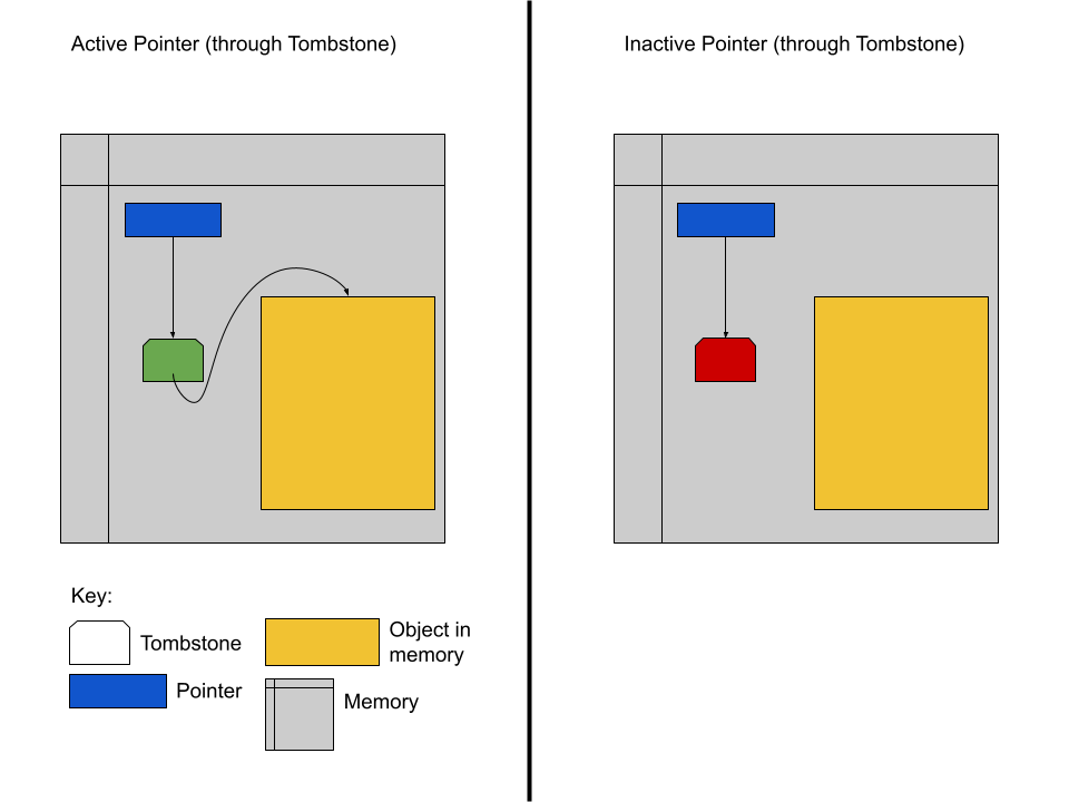
With this technique, there is no additional memory access – that’s good! However, there are still downsides. First, there is a speed cost. For every dereference there must be a check of the equality of the keys. Depending on the length of the key that can take a significant amount of time. Second, there is a space cost. Every pointer and block of allocated memory now must have enough space to store the key. For systems where memory allocations are done in big chunks, the relative size overhead of storing, say, and 8byte key is not significant. However, if the system allocates many small areas of memory, the relative size overhead is tremendous. Moreover, the more heavily the system relies on pointers the more space will be used to store keys rather than meaningful data.

Well, let’s just make the keys smaller? Great idea. There’s only one problem: The smaller the keys the fewer unique key values. Fewer unique key values mean that it is more likely an invalid pointer randomly points to a chunk of memory with a matching key. In this scenario, the protection afforded by the scheme is vitiated. (I just wanted to type that word – I’m not even sure I am using it correctly!)

10/6/2021

Original is here.

I love Reese’s Pieces.

Corrections

None to speak of!!

Pointers for Dynamic Memory Management

We finished up our discussion of pointers in today’s class. In the previous class, we talked about how pointers have two important roles in programming languages:

indirection – referring to other objects
dynamic memory management – “handles” for areas of memory that are dynamically allocated and deallocated by the system.

On Monday we focused on the role of pointers in indirection and how to solve some of the problems that can arise from using pointers in that capacity. In today’s class, we focused on the role of pointers in dynamic memory management.

As tools for dynamic memory management, the programmer can use pointers to target blocks (N.B.: I am using blocks as a generic term for memory and am not using it in the sense of a block [a.k.a. page] as defined in the context of operating systems) of dynamic memory that are allocated and deallocated by the operating system for use by an application. The programmer can use these pointers to manipulate what is stored in those blocks and, ultimately, release them back to the operating system when they are no longer needed.

Memory in the system is a finite resource. If a program repeatedly asks for memory from the system without releasing previous allocations back to the system, there will come a time when the memory is exhausted. In order to be able to release existing allocations back to the operating system for reuse by other applications, the programmer must not lose track of those existing allocations. When there is a memory allocation from the operating system to the application that can no longer be reached by a pointer in the application, that memory allocation is leaked. Because the application no longer has a pointer to it, there is no way for the application to release it back to the system. Leaked memory belongs to the leaking application until it terminates.

For some programs this is fine. Some applications run for a short, defined period of time. However, there are other programs (especially servers) that are written specifically to operate for extended periods of time. If such applications leak memory, they run the risk of exhausting the system’s memory resources and failing (Links to an external site.).

Preventing Memory Leaks

System behavior will be constrained when those systems are written in languages that do not support using pointers for dynamic memory management. However, what we learned (above) is that it is not always easy to use pointers for dynamic memory management correctly. What are some of the tools that programming languages provide to help the programmer manage pointers in their role as managers of dynamic memory.

Reference Counting

In a reference-counted memory management system, each allocated block of memory given to the application by the system contains a reference count. That reference count, well, counts the number of references to the object. In other words, for every pointer to an operating-system allocated block of memory, the reference count on that block increases. Every time that a pointer’s target is changed, the programming language updates the reference counts of the old target (decrement) and the new target (increment), if there is a new target (the pointer could be changed to null, in which case there is no new target). When a block’s reference count reaches zero, the language knows that the block is no longer needed, and automatically returns it to the system! Pretty cool.

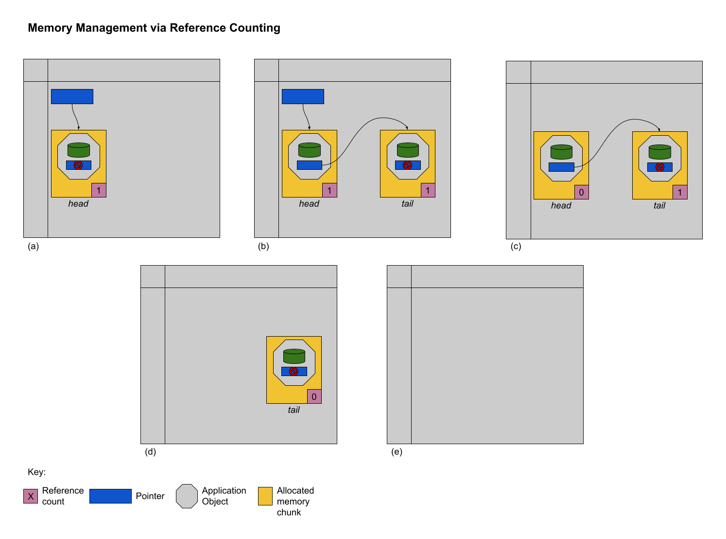
The scenario depicted visually shows the reference counting process. At time (a), the programmer allocates a block of memory dynamically from the operating system and puts an application object in that block. Assume that the application object is a node in a linked list. The first node is the head of the list. Because the programmer has a pointer that targets that allocation, the block’s reference count at time (a) is 1. At time (b), the programmer allocates a second block of memory dynamically from the system and puts a second application object in that block – another node in the linked list (the tail of the list). Because the head of the list is referencing the tail of the list, the reference count of the tail is 1. At time (c) the programmer deletes their pointer (or reassigns it to a different target) to the head of the linked list. The programming language decrements the reference count of the block of memory holding the head node and deallocates it because the reference count has dropped to 0. Transitively, the pointer from the head application object to the tail application object is deleted and the programming language decrements the reference count of its target, the block of memory holding the tail application object (time (d)). The reference count of the block of memory holding the tail application object is now 0 and so the programming language automatically deallocates the associated storage (time (e)). Voila – an automatic way to handle dynamic memory management.

There’s only one problem. What if the programmer wants to implement a circularly linked list?

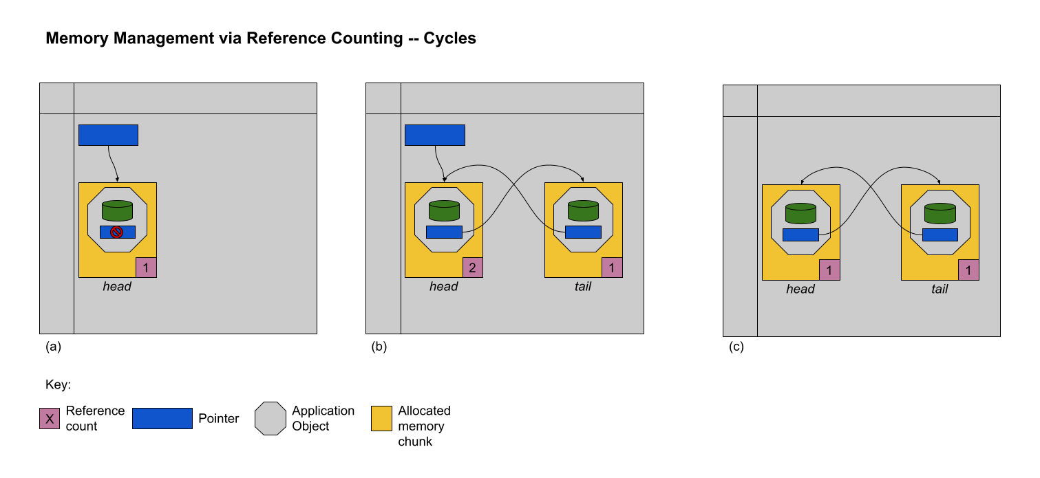
Because the tail node points to the head node, and the head node points to the tail node, even after the programmer’s pointer to the head node is deleted or retargeted, the reference counts of the two nodes will never drop to 0. In other words, even with reference-counted automatic memory management, there could still be a memory leak! Although there are algorithms to break these cycles, it’s important to remember that reference counting is not a panacea. Python is a language that manages memory using reference counting.

Garbage Collection

Garbage collection (GC) is another method of automatically managing dynamically allocated memory. In a GC’d system, when a programmer allocates memory to store an object and no space is available, the programming language will stop the execution of the program (a so-called GC pause) to calculate which previously allocated memory blocks are no longer in use and can be returned to the system. Having freed up space as a result of cleaning up unused garbage, the allocation requested by the programmer can be satisfied and the execution of the program can continue.

The most efficient way to engineer a GC’d system is if the programming language allocates memory to the programmer in fixed-size cells. In this scenario, every allocation request from the programmer is satisfied by a block of memory from one of several banks of fixed-size blocks that are stacked back-to-back. For example, a programming language may manage three different banks – one that holds reserves of X-sized blocks, one that holds reserves of Y-sized blocks and one that holds reserves of Z-sized blocks. When the programmer asks for memory to hold an object that is of size a, the programming language will deliver a block that is just big enough to that object. Because the size of the requested allocation may not be exactly the same size as one of the available fixed-size blocks, space may be wasted.

The fixed sizing of blocks in a GC’d system makes it easy/fast to walk through every block of memory. We will see shortly that the GC algorithm requires such an operation every time that it stops the program to do a cleanup. Without a consistent size, traversing the memory blocks would require that each block hold a tag indicating its size – a waste of space and the cause of an additional memory read – so that the algorithm could dynamically calculate the starting address of the next block.

When the programmer requests an allocation that cannot be satisfied, the programming language stops the execution of the program and does a garbage collection. The classic GC algorithm is called mark and sweep and has three steps:

Every block of memory is marked as free using a free bit attached to the block. Of course, this is only true of some of the blocks, but the GC is optimistic! All pointers active at the time the program is paused are traced to their targets. The free bits of those blocks are reset. The blocks that are marked free and released.

The process is shown visually below:

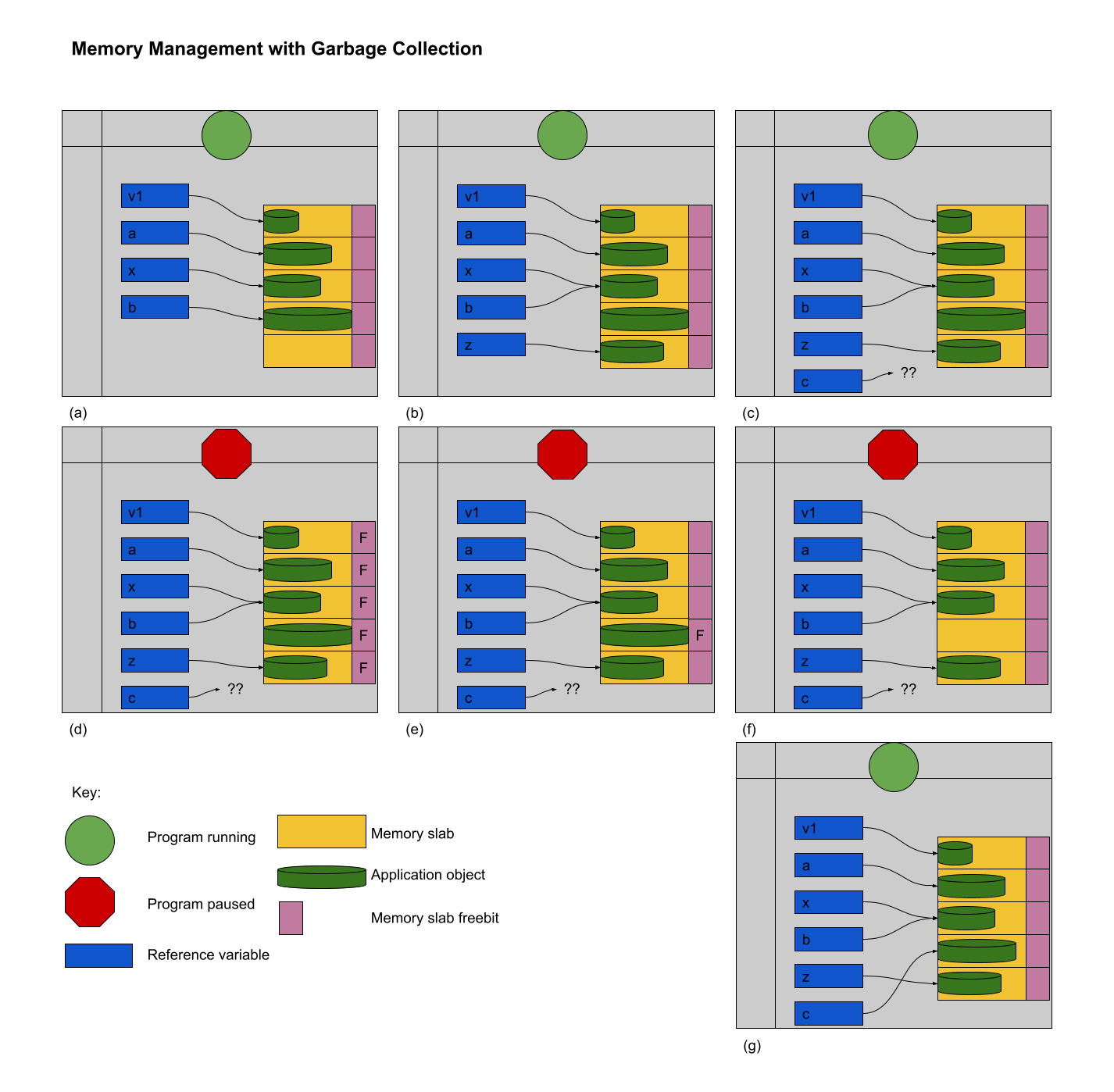
At times (a), (b) and (c), the programmer is allocating and manipulating references to dynamically allocated memory. At time (c), the allocation request for variable z cannot be satisfied because there are no available blocks. A GC pause starts at time (d) and the mark-and-sweep algorithm commences by setting the free bit of every block. At time (e) the pointers are traced and the appropriate free bits are cleared. At time (f) the memory is released from the unused block and its free bit, too, is reset. At time (g) the allocation for variable z can be satisfied, the GC pause completes and the programming language restarts execution of the program.

This process seems great, just like reference counting seemed great. However, there is a significant problem: The programmer cannot predict when GC pauses will occur and the programmer cannot predict how long those pauses will take. A GC pause is completely initiated by the programming language and (usually) completely beyond the control of the programmer. Such random pauses of program execution could be extremely harmful to a system that is controlling a system that needs to keep up with interactions from the outside world. For instance, it would be totally unacceptable for an autopilot system to take an extremely long GC pause as it calculates the heading needed to land a plane. There are myriad other systems where pauses are inappropriate.

The mark-and-sweep algorithm described above is extremely naive and GC algorithms are the subject of intense research. Languages like go and Java manage memory with a GC and their algorithms are incredibly sophisticated. If you want to know more, please let me know!

10/15/2021

The hunt for October!

Corrections

None to speak of!!

Introduction to Functional Programming

We spent Friday beginning our module on Functional Programming (FP)! As we said at the beginning of the semester when we were learning about programming paradigms, FP is very different than imperative programming. In imperative programming, developers tell the computer how to do the operation. While functional programming is not logic programming (where developers just tell the computer what to compute and leave the how entirely to the language implementation), the writer of a program in a functional PL is much more concerned with specifying what to compute than how to compute it.

Four Characteristics of Functional Programming

There are four characteristics that epitomize FP:

There is no state
Functions are central
1. Functions can be parameters to other functions
2. Functions can be return values from other others
3. Program execution is function evaluation
Control flow is performed by recursion and conditional expressions
Lists are a fundamental data type

In a functional programming language, there are no variables, per se. And because there are no variables, there is no state. That does not mean there are no names. Names are still important. It simply means that names refer to expressions themselves and not their values. The distinction will become more obvious as we continue to learn more about writing programs in functional languages.

Because there is no state, a functional programming language is not history sensitive. A language that is history sensitive means that results of operations in that language can be affected by operations that have come before it. For example, in an imperative programming language, a function may be history sensitive if it relies on the value of a global variable to calculate its return value. Why does that count as history sensitive? Because the value in the global variable could be affected by prior operations.

A language that is not history sensitive has referential transparency. We learned the definition of referential transparency before, but now it might make a little more sense. In a language that has referential transparency, a the same function called with the same arguments generates the same result no matter what operations have preceded it.

In a functional programming language there are no loops (unless they are added as syntactic sugar) – recursion is the way to accomplish repetition. Selective execution (as opposed to sequential execution) is accomplished using the conditional expression. A conditional expression is, well, an expression that evaluates to one of two values depending on the value of a condition. We have seen conditional expressions in STIMPL. That a conditional statement can have a value (thus making it a conditional expression) is relatively surprising for people who only have experience in imperative programming languages. Nevertheless, the conditional expressions is a very, very sharp sword in the sheath of the functional programmer.

A functional program is a series of functions and the execution of a functional program is simply an evaluation of those functions. That sounds abstract at this point, but will become more clear when we see some real functional programs.

Lists are a fundamental data type in functional programming languages. Powerful syntactic tools for manipulating lists are built in to most functional PLs. Understanding how to wield these tools effectively is vital for writing code in functional PLs.

The Historical Setting of the Development of Functional PLs

The first functional programming language was developed in the mid-1950s by John McCarthy . At the time, computing was most associated with mathematical calculations. McCarthy was instead focused on artificial intelligence which involved symbolic computing. Computer scientists thought that it was possible to represent cognitive processes as lists of symbols. A language that made it possible to process those lists would allow developers to build systems that work like our brains.

McCarthy started with the goal of writing a system of meta notation that programmers could attach to Fortran. These meta notations would be reduced to actual Fortran programs. As they did their work, they found their way to a program representation built entirely of lists (and lists of lists, and lists of lists of lists, etc). Their thinking resulted in the development of Lisp, a list processing language. In Lisp, data are lists and programs are lists. They showed that list processing, the basis of the semantics of Lisp, is capable of universal computing. In other words, Lisp, and other list processing languages, is/are Turing complete.

The inability to execute a Lisp program efficiently on a physical computer based on the von Neumann model has given Lisp (and other functional programming languages) a reputation as slow and wasteful. (N.B.: This is not true today!) Until the late 1980s hardware vendors thought that it would be worthwhile to build physical machines with non-von Neumann architectures that made executing Lisp programs faster. Here is an image of a so-called Lisp Machine.

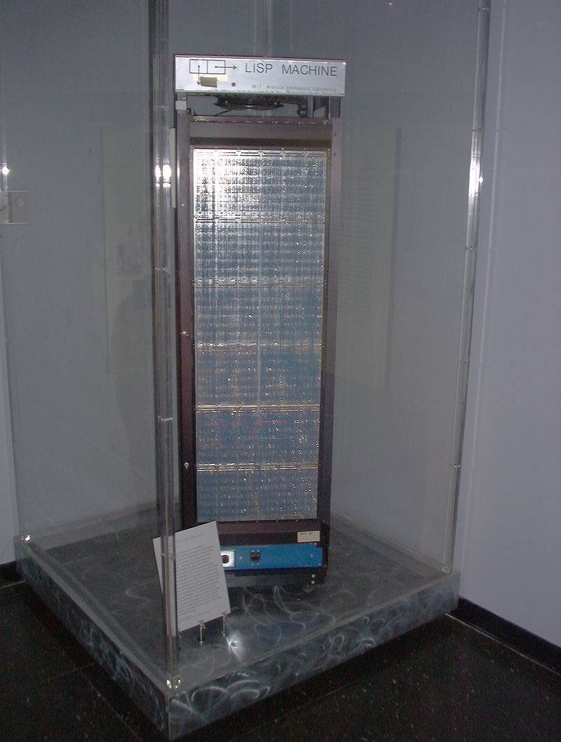
LISP

We will not study Lisp in this course. However, there are a few aspects of Lisp that you should know because they pervade the general field of computer science.

First, you should know CAR, CDR and CONS – pronounced car, could-er, and cahns, respectively. CAR is a function that takes a list as a parameter and returns the first element of the list. CDR is a function that takes a list as a parameter and returns the tail, everything but the head, of the list. CONS takes two parameters – a single element and a list – and returns a new list with the first argument appended to the front of the second argument.

For instance,

(car (1 2 3))

is 1.

(cdr (1 2 3))

is (2 3).

Second, you should know that, in Lisp, all data are lists and programs are lists.

(a b c)

is a list in Lisp. In Lisp, (a b c) could be interpreted as a list of atoms a, b and c or an invocation of function a with parameters b and c.

Lambda Calculus

Lambda Calculus is the theoretical basis of functional programming languages in the same way that the Turing Machine is the theoretical basis of the imperative programming languages. The Lambda Calculus is nothing like “calculus” – the word calculus is used here in its strict sense: a method or system of calculation . It is better to think of Lambda Calculus as a programming language rather than a branch of mathematics.

Lambda Calculus is a model of computation defined entirely by function application. The Lambda Calculus is as powerful as a Turning Machine which means that anything computable can be computed in the Lambda Calculus. For a language as simple as the Lambda Calculus, that’s remarkable!

The entirety of the Lambda Calculus is made up of three entities:

Expression: a name, a function or an application
Function: \(\lambda\) .
Application:

Notice how the elements of the Lambda Calculus are defined in terms of themselves. In most cases it is possible to restrict names in the Lambda Calculus to be any single letter of the alphabet – a is a name, z is a name, etc. Strictly speaking, functions in the Lambda Calculus are anonymous – in other words they have no name. The name after the

in a function in the Lambda Calculus can be thought of as the parameter of the function. Here’s an example of a function in the Lambda Calculus:

\(\lambda\)x . x

Lambda Calculiticians (yes, I just made up that term) refer to this as the identity function. This function simply returns the value of its argument! But didn’t I say that functions in the Lambda Calculus don’t have names? Yes, I did. Within the language there is no way to name a function. That does not mean that we cannot assign semantic values to those functions. In fact, associating meaning with functions of a certain format is exactly how high-level computing is done with the Lambda Calculus.

10/18/2021

Lambda lower now. How low can you go?

Corrections

None to speak of!!

(Recalling) Lambda Calculus

Remember that we said Lambda Calculus is the theoretical basis of functional programming languages in the same way that the Turing Machine is the theoretical basis of the imperative programming languages. Again, don’t freak out when you hear the phrase “calculus”. As we said in class, it is better to think of the Lambda Calculus as a programming language rather than a branch of mathematics.

Remember that the entirety of the Lambda Calculus is made up of a small number of entities:

Expression: a name, a function or an application
Function: \(\lambda\) .
Application:

We made the point in class that, without loss of generality, we will assume that all names are single letters from the alphabet. In other words, if you see two consecutive letters, e.g., ab, those are two separate names.

Bound and Free Names and the Tao of Function Application

Because the entirety of the Lambda Calculus is function application, it is important that we get it exactly right. Let’s recall the simplest example of function application: \((\lambda a. a)x = \left \lfloor x/a \right \rfloor a = x\) The \(\lfloor x/a \rfloor a\) means “replace all instances of a with x in whatever comes after the \(\lfloor \rfloor\) “. This is so easy. What about this, though?

\((\lambda a. \lambda b. ba)b\)

The first thing to realize is that the b in the expression that is the body of the nested lambda function is completely separate from the b to which the lambda function is being applied. Why is that? Because the b in the nested lambda function is the “parameter” to that function. So, what are we to do?

First, let’s step back and consider the definitions of free and bound names. Loosely speaking, a name is bound as soon as it is used as a parameter to a lambda function. It continues to be bound in nested expressions but may be rebound! For example,

\(\lambda x. x \lambda x. x\)

The “body” of the outer function is \(x \lambda x . x\) and the leftmost x is the x from the outer function’s parameter. In other words,

\((\lambda x.x \lambda x.x) (a) = a \lambda x.x\)

The substitution of a for x continues no further because x is rebound at the start of the nested lambda function. You will be relieved to know that,

\(\lambda x.x \lambda x.x = \lambda x.x \lambda a.a\)

In fact, renaming like that has a special name: alpha conversion!

Free names are those that are not bound.

Wow, that got pretty complicated pretty quickly! This is one case where some formalism actually improves the clarity of things, I think. Here is the formal definition of what it means for a name to be bound:

name is bound in \(\lambda name_1.expression\) if name = name1 or name is bound in expression.
name is bound in \(E_1 E_2\) if name is bound in either \(E_1\) or \(E_2\).

Here is the formal definition of what it means for a name to be free:

name is free in name
name is free in \(\lambda name_1.expression\) when name \(\ne\) name1 and name is free in expression
name is free in \(E_1E_2\) if name is free in either E1 or E2

Note that a name can be free and bound at the same time.

All this hullabaloo means that we need to be slightly more sophisticated in our function application. We have to check two boxes before assuming that can treat function application as a simple textual search/replace:

When applying \(\lambda x. E_1\) to E2, we only replace the free instances of x in E1 with E2 and if E2 contains a free name that is bound in E1, we have to alpha convert that bound name in E1 to something that doesn’t conflict. There is a good example of this in Section 1.2 of the XXXX that I will recreate here:

\((\lambda x. (\lambda y . (x\lambda x. xy)))y\)

First, note y (our E2 in this case) contains y (a free name) that is bound in \((\lambda y. (x \lambda x.xy))\)(our E1). In other words, before doing a straight substitution, we have to alpha convert the bound y in E1 to something that doesn’t conflict. Let’s choose t:

\((\lambda x. (\lambda t. (x \lambda x.xt)))y\)

Now we can do our substitution! But, be careful: x appears free in \((\lambda y. (x \lambda x.xy)\) (again, our E1) one time – its leftmost appearance! So, the substitution would yield:

\((\lambda t. (y \lambda x.xt)\)

Voila!

Currying Functions

Currying is the process of turning a function that takes multiple parameters into a sequence of functions that each take a single parameter. Currying is only possible in languages that support high-order functions: functions that a) take functions as parameters, b) return functions or c) both. Python is such a language. Let’s look at how you would write a function that calculates the sum of three numbers in Python:

def sum3(a, b, c):
  return a + b + c

That makes perfect sense!

Let’s see if we can Curry that function. Because a Curried function can only take one parameter and we are Currying a function with three parameters, it stands to reason that we are going to have to generate three different functions. Let’s start with the first:

def sum1(a):
  # Something?

What something are we going to do? Well, we are going to declare another function inside sum1, call it sum2, that takes a parameter and then use that as the return value of sum1! It looks something like this:

def sum1(a):
  def sum2(b):
    pass
  return sum2

That means, if we call sum1 with a single parameter, the result is another function, one that takes a single parameter! So, we’ve knocked off two of the three parameters, now we need one more. So, let’s write something like this:

def sum1(a):
  def sum2(b):
    def sum3(c):
      pass
    return sum3
  return sum2

This means that if we call sum1 with a single parameter and call the result of that with a single parameter, the result is another function, one that also takes a single parameter! What do we want that innermost function to do? That’s right: the summation! So, here’s our final code:

def sum1(a):
  def sum2(b):
    def sum3(c):
      return a + b + c
    return sum3
  return sum2

We’ve successfully Curried a three-parameter summation function! There’s just one issue left to address? How can we possibly use a and b in the innermost function? Will, I thought you told us that Python was statically scoped! In order for this to work correctly, wouldn’t Python have to have something magical and dynamic-scope-like? Well, yes! And, it does. It has closures.

When you return sum2 from the body of sum1, Python closes around the variables that are needed by any code in the implementation of the returned function. Because a is needed in the implementation of sum2 (the function returned by sum1), Python creates a closure around that function which includes the value of a at the time sum2 was returned. It is important to remember that every time sum2 is defined pursuant to an invocation of sum1, a new version of sum2 is returned with a new closure. This closure-creation process repeats when we return sum3 pursuant to an invocation of sum2 (which itself was generated as a result of an invocation of sum1)! Whew.

Because we Curried the sum3 function as sum1, we have to call them slightly differently:

  sum3(1, 2, 3)
  sum1(1)(2)(3)

As we learn more about functional programming in Haskell, you will see this pattern more and more and it will become second nature.

The “good” news, if you can call it that, is that functions in the Lambda Calculus always exist in their Curried form. Prove it to yourself by looking back at the way we formally defined the Lambda Calculus.

But, because it is laborious to write all those \(\lambda\)s over and over, we will introduce a shorthand for functions in the Lambda Calculus that take more than one parameter:

\(\lambda p_1p_2 … p_n.expression\)

is a function with n parameters named p1 through pn (which are each one letter). Simply put,

\(\lambda x . \lambda y.xy = \lambda xy.xy\)

for example.

Doing Something with Lambda Calculus

Remember how we have stressed that you cannot name functions inside the Lambda Calculus but how I have stressed that does not mean we cannot give names to functions from outside the Lambda Calculus? Well, here’s where it starts to pay off! We are going learn how to do boolean operations using the Lambda Calculus. Let’s assume that anytime we see a lambda function that takes two parameters and reduces to the first, we call that T. When we see a lambda function that takes two parameters and reduces to the second, we call that F:

\(T \equiv \lambda xy.x\)

\(F \equiv \lambda xy.y\)

To reiterate, it is the form that matters. If we see

\(\lambda ab.a\)

that is T too! In what follows, I will type T and F to save myself from writing all those \(\lambda\)s, but remember: T and F are just functions!!

Okay, let’s do something boolean operations. We can define the and operation as

\(\wedge = \lambda xy.xy F\)

Let’s give it a whirl. First, let’s get on the same page: True and False is False.

\(\wedge TF = (\lambda xy.xyF)TF = TFF = (\lambda xy.x) FF = F\)

Awesome! Let’s try another: True and True is True.

\(\wedge TT = (\lambda xy.xyF)TT = TTF = (\lambda xy.x) TF = T\)

We can define the or operation as

\(\lor = \lambda xy.xTy\)

Try your hand at working through a few examples and make sure you get the expected results!

10/22/2021

Corrections

Thanks to Donald’s persistence, I researched the mechanism by which Haskell and other pure functional languages

handle associations between names and expressions, and
pass around infinite lists (without having to generate the entire list first – an obvious impossibility)

thunks are covered below!

Function Invocation in Functional Programming Languages

In imperative programming languages, it may matter to the correctness of a program the order in which parameters to a function are evaluated. (Note: For the purposes of this discussion we will assume that all operators [+, -, /, etc] are implemented as functions that take the operands as arguments in order to simplify the discussion. In other words, when describe the order of function evaluation we are also talking about the order of operand evaluation.) While the choice of the order in which we evaluate the operands is the language designer’s prerogative, the choice has consequences. Why? Because of side effects! For example:

#include <stdio.h>

int operation(int parameter) {
  static int divisor = 1;
  return parameter / (divisor++);
}

int main() {
  int result = operation(5) + operation(2);
  printf("result: %d\n", result);
  return 0;
}

prints

result: 6

whereas

#include <stdio.h>

int operation(int parameter) {
  static int divisor = 1;
  return parameter / (divisor++);
}

int main() {
  int result = operation(2) + operation(5);
  printf("result: %d\n", result);
  return 0;
}

prints

result: 4

In the difference between the two programs we see vividly the role that the static variable plays in the state of the program and its ultimate output.

Because of the referential transparency in pure functional programming languages, the designer of such a language does not need to worry about the consequences of the decision about the order of evaluation of arguments to functions. However, that does not mean that the language designer of a pure functional programming language does not have choices to make in this area.

A very important choice the designer has to make is the time when function arguments are evaluated. There are two options available:

All function arguments are evaluated before the function is evaluated.
Function arguments are evaluated only when their results are needed.

Let’s look at an example: Assume that there are two functions: dbl, a function that doubles its input, and average, a function that averages its three parameters:

dbl x = (+) x x
average a b c = (/) ((+) a ((+) b c)) 3

Both functions are written using prefix notation (i.e., ( … ). We will call these functions like this:

dbl (average 3 4 5)

If the language designer chooses to evaluate function arguments only when their results are needed, the execution of this function call proceeds as follows:

dbl (average 3 4 5)
+ (average 3 4 5) (average 3 4 5)
+ ((/) ((+) 3 ((+) 4 5)) 3) (average 3 4 5)
+ (4) (average 3 4 5)
+ (4) ((/) ((+) 3 ((+) 4 5)) 3)
+ (4) (4)
8

The outermost function is always reduced (expand) before the inner functions. Note: Primitive functions (+, and / in this example) cannot be expanded further so we move inward in evaluation if we encounter such a function for reduction.

If, however, the language designer chooses to evaluate function arguments before the function is evaluated, the execution of the function call proceeds as follows:

dbl (average 3 4 5)
dbl ((/) ((+) 3 ((+) 4 5)) 3)
dbl 4
+ 4 4
8

No matter the designer’s choice, the outcome of the evaluation is the same. However, there is something strikingly different about the two. Notice that in the first derivation, the calculation of the average of the three numbers happens twice. In the second derivation, it happens only once! That efficiency is not a fluke! Generally speaking, the method of function invocation where arguments are evaluated before the function is evaluated is faster.

These two techniques have technical names:

applicative order: “all the arguments to … procedures are evaluated when the procedure is applied.”
normal order: “delay evaluation of procedure arguments until the actual argument values are needed.”

These definitions come from

Abelson, H., Sussman, G. J.,, with Julie Sussman (1996). Structure and Interpretation of Computer Programs. Cambridge: MIT Press/McGraw-Hill. ISBN: 0-262-01153-0

It is obvious, then, that any serious language designer would choose applicative order for their language. There’s no reason redeeming value for the inefficiency of normal order. The Implications of Applicative Order

Scheme is a Lisp dialect . I told you that we weren’t going to work much with Lisp, but I lied. Sort of. Scheme is an applicative-order language with the same list-is-everything syntax as all other Lisps (see The Daily PL - 10/15/2021). In Scheme, you would define an if function named myif like this:

(define (myif c t f) (cond (c t) (else f)))

c is a boolean and myif returns t when c is true and f when c is false. No surprises.

We can define a name a and set its value to 5:

(define a 5)

Now, let’s call myif:

(myif (= a 0) 1 (/ 1 a))

If a is equal to 0, then the call returns 1. Perfect. If a is not zero, the call returns the reciprocal of a. Given the value of a, the result is 1/7.

Let’s define the name b and set its value to 0:

(define b 0)

Now, let’s call myif:

(myif (= b 0) 1 (/ 1 b))

If b is equal to 0, then the call returns 1. If b is not zero, the call returns the reciprocal of b. Given the value of b, the result is 1:

/: division by zero
  context...:
   "/home/hawkinsw/code/uc/cs3003/scheme/applicative/applicative.rkt": [running body]
   temp37_0
   for-loop
   run-module-instance!125
   perform-require!78

That looks exactly like 1. What happened?

Remember we said that the language is applicative order. No matter what the value of b, both of the arguments are going to be evaluated before myif starts. Therefore, Scheme attempts to evaluate 1 / b which is 1 / 0 which is division by zero.

Thanks to situations like this, the Scheme programming language is forced into defining special semantics for certain functions, like the built-in if expression. As a result, function invocation is not orthogonal in Scheme – the general rules of function evaluation in Scheme must make an exception for applying functions like the built-in if expression. Remember that the orthogonality decreases as exceptions in a language’s specification increase. Sidebar: Solving the problem in Scheme

Feel free to skip this section if you are not interested in details of the Scheme programming language. That said, the concepts in this section are applicable to other languages.

In Scheme, you can specify that the evaluation of an expression be delayed until it is forced.

(define d (delay (/ 1 7)))

defines d to be the eventual result of the evaluation of the division of 1 by 7. If we ask Scheme to print out d, we see

#<promise:d>

To bring the future tense into the present tense, we force a delayed evaluation:

(force d)

If we ask Scheme to print the result of that expression, we see:

1/7

Exactly what we expect! With this newfound knowledge, we can rewrite the myif function:

(define (myif c t f) (cond (c (force t)) (else (force f))))

Now myif can accept ts and fs that are delayed and we can use myif safely:

(define b 0)
(myif (= b 0) (delay 1) (delay (/ 1 b)))
#+end_src lisp

and we see the reasonable result:
#+begin_src
1

Kotlin, a modern language, has a concept similar to delay called lazy . Ocaml, an object-oriented functional programming language, contains the same concept . Swift has some sense of laziness , too!

Well, We Are Back to Normal Order

I guess that we are stuck with the inefficiency inherent in the normal order function application. Going back to the dbl/average example, we will just have to live with invoking average twice.

Or will we?

Real-world functional programming languages that are normal order use an interesting optimization to avoid these recalculations! When an expression is passed around and it is unevaluated, Haskell and languages like it represent it as a thunk (Links to an external site.). The thunk data structure is generated in such a way that it can calculate the value of its associated expression some time in the future when the value is needed. Additionally, the thunk then caches (or memoizes) the value so that future evaluations of the associated expression do not need to be repeated.

As a result, in the dbl/average example,

a thunk is created for (average 3 4 5),
that thunk is passed to dbl, where it is duplicated during the reduction of dbl,
(average 3 4 5) is (eventually) calculated for the first time using the thunk,
4 is stored (cached, memoized) in the thunk, and
the cached/memoized value is retrieved from the thunk instead of evaluating (average 3 4 5) for a second time.

A thunk, then, is the mechanism that allows the programmer to have the efficiency of applicative order function invocation with the semantics of the normal order function invocation!

10/27/2021

The Tail That Wags the Dog

There are no loops in functional programming languages. We’ve learned that, instead, functional programming languages are characterised by the fact that they use recursion for control flow. As we discussed earlier in the class (much earlier, in fact), when running code on a von Neumann machine, iterative algorithms typically perform faster than recursive algorithms because of the way that the former leverages the properties of the hardware (e.g., spatial and temporal locality of code ). In addition, recursive algorithms typically use much more memory than iterative algorithms.

Why? To answer that question, we will need to recall what we learned about stack frames. For every function invocation, an activation record (aka stack frame) is allocated on the run-time stack (aka call stack). The function’s parameters, local variables, and return value are all stored in its activation record. The activation record for a function invocation remains on the stack until it has completed execution. In other words, if a function f invokes a function g, then function f’s activation record remains on the stack until (at least) g has completed execution.

Consider some algorithm A. Let’s assume that an iterative implementation of A requires n executions of a loop and l local integer variables. If that implementation is contained in a function, an invocation of that function would consume approximately l*sizeof(integer variable) + activation record overhead space on the runtime stack. Let’s further assume that a function implementing the recursive version of A also uses l local integer variables and also requires n executions of itself. Each invocation of the implementing function, then, needs l*sizeof(integer variable) + activation record overhead space on the runtime stack. Multiply that by n, the number of recursive calls, and you can see that, at it’s peak, executing the recursive version of algorithm A requires n * (l * sizeof(integer variable) + activation record overhead) space on the run-time stack. In other words, the recursive version requires n times more memory! That escalated quickly .

That’s all very abstract. Let’s look at the implications with a real-world example, which we will write in Haskell syntax:

myLen [] = 0
myLen (x:xs) = 1 + (myLen xs)

myLen is a function that recursively calculates the length of a list. Let’s see what the stack would look like when we call myLen [1,2,3]:

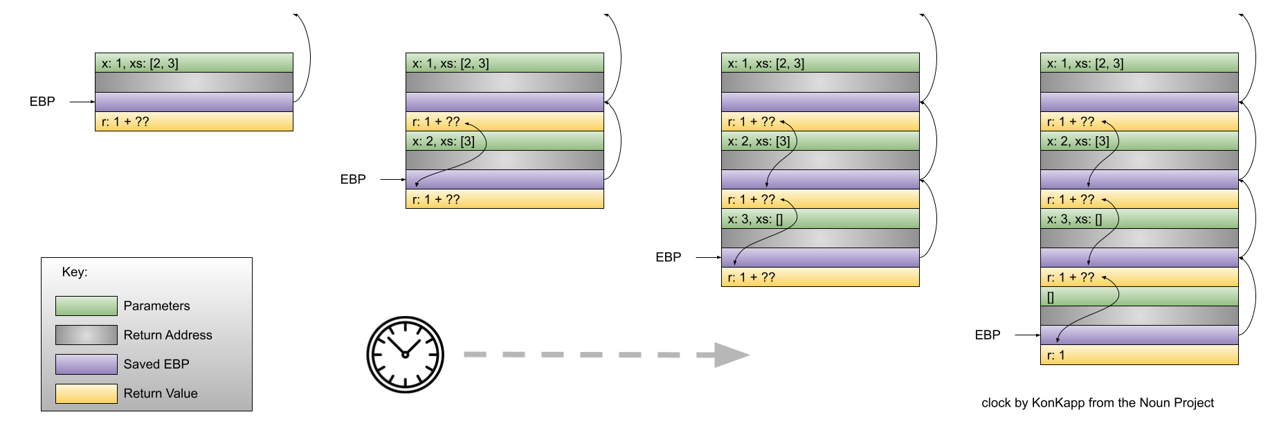
When the recursive implementation of myLen reaches the base case, there are four activation records on the run-time stack.

Allocating space on the stack takes time. Therefore, the more activation records placed on the stack, the more time the program will take to execute. But, if we are willing to live with a slower program, then there’s nothing else to worry about.

Right?

Wrong. Modern hardware is fast. Modern computers have lots of memory. Unfortunately, they don’t have an infinite amount of memory. A program only has a finite amount of stack space. Given a long enough list, myLen could cause so many activation records to be placed on the stack that the amount of stack space is exhausted and the program crashes. In other words, it’s not just that a recursive algorithm might execute slower, a recursive algorithm might fail to calculate the correct result entirely!

Tail Recursion - Hope

The activation records of functions that recursively call themselves remain on the stack because, presumably, they need the result of the recursive invocation to complete their work. For example, in our myLen function, an invocation of myLen cannot completely calculate the length of the list given as a parameter until the recursive call completes.

What if there was some way to rewrite a recursive function in a way that it did not need to wait on a future recursive invocation to completely calculate its result? If that could happen, then the stack frame of the current invocation of the function could be replaced by the stack frame of the recursive invocation. Why? Because the information contained in the current invocation of the function has no bearing on its overall result – the only information needed to completely calculate the result of the function is the result of the future recursive invocation! The implementation of a recursive function that matches this specification is known as a tail-recursive function. The book says “A function is tail recursive if its recursive call is the last operation in the function.”

With a tail-recursive function, we get the expressiveness of a recursive definition of the algorithm along with the efficiency of an iterative solution! Ron Popeil, that’s a deal!

Rewriting

The rub is that we need to figure out a way to rewrite those non-tail recursive functions into tail-recursive versions. I am not aware of any general purpose algorithms for such a conversion. However, there is one technique that is widely applicable: accumulators. It is sometimes possible to add a parameter to a non-tail recursive function and use that parameter to define a tail-recursive version. Seeing an accumulator in action is the easiest way to define the technique. Let’s rewrite myLen in a tail-recursive manner using an accumulator:

myLen list = myLenImpl 0 list
myLenImpl acc [] = acc
myLenImpl acc (x:xs) = myLenImpl (1 + acc) xs

First, notice how we are turning myLen into a function that simply invokes a worker function whose job is to do the actual calculation! The first parameter to myLenImpl is used to hold a running tally of the length of the list so far. The first invocation of myLenImpl from the implementation of myLen, then, passes 0 as the argument to the accumulator because the running tally of the length so far is, well, 0. The implementation of myLenImpl adds 1 to that accumulator variable for every list item that is stripped from the front of the list. The result is that the result of an invocation of myLenImpl does not rely on the completion of a recursive execution. Therefore, myLenImpl qualifies as a tail-recursive function! Woah.

Let’s look at the difference in the contents of the run-time stack when we use the tail-recursive version of myLen to calculate the length of the list [1,2,3]:

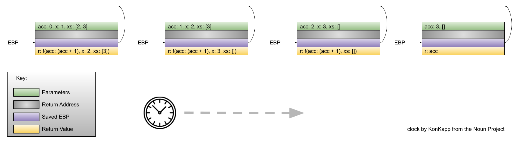
A constant amount of stack space is being used – amazing!

10/29/2021

No one Puts Locals In a Corner

One of the really cool things about functional programming languages is their first-class support for functions. In functional programming languages, the programmer can pass functions as parameters to other functions and return functions from functions. Let’s take a closer look at functions that “generate” other functions. JavaScript has the capability to return functions from functions so we’ll use that language to explore:

function urlGenerator(prefix) {
  function return_function(url) {
    return prefix + "://" + url;
  }
  return return_function;
}

The urlGenerator function takes a single parameter – prefix. The caller of urlGenerator passes the protocol prefix as the argument (probably either “http” or “https”). The return value of urlGenerator is itself a function that takes a single parameter, a url, and returns url prepended with the prefix specified by the call to urlGenerator. An example might help:

const httpsUrlGenerator = urlGenerator("https");
const httpUrlGenerator = urlGenerator("http");

console.log(httpsUrlGenerator("google.com"));
console.log(httpUrlGenerator("google.com"));

generates

"https://google.com"
"http://google.com"

In other words, the definition of httpsUrlGenerator is (conceptually)

  function httpsUrlGenerator(url) {
    return "https" + "://" + url;
  }

and the definition of httpUrlGenerator is (conceptually)

  function httpUrlGenerator(url) {
    return "http" + "://" + url;
  }

But that’s only a conceptual definition! The real definition continues to contain prefix:

    return prefix + "://" + url;

But, prefix is locally scoped to the urlGenerator function. So, how can httpUrlGenerator and httpsUrlGenerator continue to use its value after leaving the scope of urlGenerator?

The Walls Are Closing In

JavaScript, and other languages like it, have the concept of closures. A closure is a context that travels with a function returned by another function. Inside the closure are values for the free variables (remember that definition?) of the returned function. In urlGenerator, the returned function (return_function) uses the free variable prefix. Therefore, the closure associated with return_function contains the value of prefix at the time the closure is created!

In the example above, there are two different copies of return_function generated – one when urlGenerator is called with the argument “http” and one when urlGenerator is called with the parameter “https”. Visually, the situation is

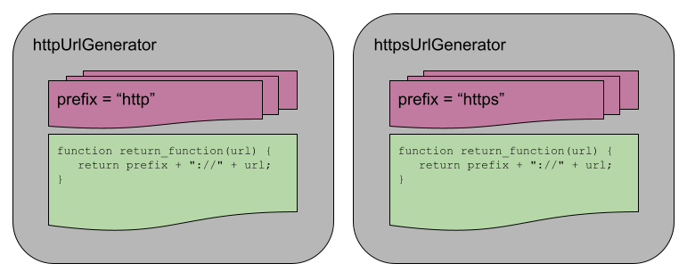
Connections with Other Material

Think about the connection between closures and the format of the urlGenerator/return_function functions and other concepts we’ve explored previously like partial application and currying.

11/1/2021

Your Total Is …

In today’s class, we started with writing a simple function to sum the numbers in a list and ended up with the definition of a fundamental operation of functional programming: the fold. Let’s start by writing the simple, recursive definition of a sum function in Haskell:

simpleSum [] = 0
simpleSum (first:rest) = first + (simpleSum rest)

When invoked with the list [1,2,3,4], the result is 10:

*Summit> simpleSum [1,2,3,4]
10

Exactly what we expected. Let’s think about our job security: The boss tells us that they want a function does “products” all the elements in the list. Okay, that’s easy:

simpleProduct [] = 1
simpleProduct (first:rest) = first * (simpleProduct rest)

When invoked with the list [1,2,3,4], the result is 24:

*Summit> simpleProduct [1,2,3,4]
24

Notice that there are only minor differences between the two functions: the value returned in the base case (0 or 1) and the operation being performed on head and the result of the recursive invocation.

I hear some of your shouting at me already: This isn’t tail recursive; you told us that tail recursive functions are important. Fine! Let’s rewrite the two functions so that they are tail recursive. We will do so using an accumulator and a helper function:

trSimpleSum list = trSimpleSumImpl 0 list
trSimpleSumImpl runningTotal [] = runningTotal
trSimpleSumImpl runningTotal (x:xs) = trSimpleSumImpl (runningTotal + x) xs

When invoked with the list [1,2,3,4], the result is 10:

*Summit> trSimpleSum [1,2,3,4]
10

And, we’ll do the same for the function that calculates the product of all the elements in the list:

trSimpleProduct list = trSimpleProductImpl 1 list
trSimpleProductImpl runningTotal [] = runningTotal
trSimpleProductImpl runningTotal (x:xs) = trSimpleProductImpl (runningTotal * x) xs

When invoked with the list [1,2,3,4], the result is 24:

*Summit> trSimpleProduct [1,2,3,4]
24

One of These Things is Just Like The Other

Notice the similarities between trSimpleSumImpl and trSimpleProductImpl. Besides the names, the only difference is really the operation that is performed on the runningTotal and the head element of the list. Because we’re using a functional programming language, what if we wanted to let the user specify that operation in terms of a function parameter? Such a function would need have to accept two arguments (the up-to-date running total and the head element) and return a new running total. For summing, we might write a sumOperation function:

sumOperation runningTotal headElement = runningTotal + headElement

Next, instead of defining trSimpleSumImpl and trSimpleProductImpl with fixed definitions of their operation, let’s define a trSimpleOpImpl that could use sumOperation:

trSimpleOpImpl runningTotal operation [] = runningTotal
trSimpleOpImpl runningTotal operation (x:xs) = trSimpleOpImpl (operation runningTotal x) operation xs

Fancy! Now, let’s use trSimpleOpImpl and sumOperation to recreate trSimpleSum from above:

trSimpleSum list = trSimpleOpImpl 0 sumOperation list

Let’s check to make sure that we get the same results: When invoked with the list [1,2,3,4], the result is 10:

*Summit> trSimpleSum [1,2,3,4]
10

To confirm our understanding of what’s going on here, let’s visualize the invocations of sumOperation necessary to complete the calculation of trSimpleSum:

sumOperation 0 1
sumOperation 1 2
sumOperation 3 3
sumOperation 6 4

Let’s do a similar thing for trSimpleProduct:

productOperation runningTotal headElement = runningTotal * headElement
trSimpleProduct list = trSimpleOpImpl 0 productOperation list

Let’s check to make sure that we get the same results: When invoked with the list [1,2,3,4], the result is 24:

*Summit> trSimpleProduct [1,2,3,4]
24

Think About the Types:

We’ve stumbled on a pretty useful pattern! Let’s look at its components:

A “driver” function (called trSimpleOpImpl) that takes three parameters: an initial value (of a particular type, T), an operation function (see below) and a list of inputs, each of which is of type T.
An operation function that takes two parameters – a running total, of some type R; an element to “accumulate” on to the running total of type T – and returns a new running total of type R.
A list of inputs, each of which is of type T.

Here are the types of those functions in Haskell:

operation function: R -> T -> R

list of inputs: [T]

driver function: T -> (R -> T -> R) -> R

Let’s play around and see what we can write using this pattern. How about a concatenation of a list of strings in to a single string?

concatenateOperation concatenatedString newString = concatenatedString ++ newString
concatenateStrings list = trSimpleOpImpl "" concatenateOperation list

(the ++ just concatenates two strings together). When we run this on [“Hello”, “,”, “World”] the result is “Hello, World”:

*Summit> concatenateStrings ["Hello", ",", "World"]
"Hello,World"

So far our Ts and Rs have been the same – integers and strings. But, the signatures indicate that they could be different types! Let’s take advantage of that! Let’s use trSimplOpImpl to write a function that returns True if every element in the list is equal to the number 1 and False otherwise. Let’s call the operation function continuesToBeAllOnes and define it like this:

continuesToBeAllOnes equalToOneSoFar maybeOne = equalToOneSoFar && (maybeOne == 1)

This function will return True if the list (to this point) has contained all ones (equalToOneSoFar) and the current element (maybeOne) is equal to one. In this case, the R is a boolean and the T is an integer. Let’s implement a function named isListAllOnes using continuesToBeAllOnes and trSimplOpImpl:

isListAllOnes list = trSimpleOpImpl True continuesToBeAllOnes list

Does it work? When invoked with the list [1,1,1,1], the result is True:

*Summit> isListAllOnes [1,1,1,1]
True

When invoked with the list [1,2,1,1], the result is False:

*Summit> isListAllOnes [1,2,1,1]
False

Naming those “operation” functions every time is getting annoying, don’t you think? I bet that we could be lazier!! Let’s rewrite isListAllOnes without specifically defining the continuesToBeAllOnes function:

isListAllOnes list = trSimpleOpImpl True (\equalToOneSoFar maybeOne -> equalToOneSoFar && (maybeOne == 1)) list

Now we are really getting functional!

I am greedy. I want to write a function that returns True if any element of the list is a one:

isAnyElementOne list = trSimpleOpImpl False (\anyOneSoFar maybeOne -> anyOneSoFar || (maybeOne == 1)) list

This is just way too much fun!

Fold the Laundry

This type of function is so much fun that it is included in the standard implementation of Haskell! It’s called fold! And, in true Haskell fashion, there are two different versions to maximize flexibility and confusion: the fold-left and fold-right operation. The signatures for the functions are the same in both cases:

fold[l,r] :: operation function -> initial value -> list -> result

In all fairness, these two versions are necessary. Why? Because certain operation functions are not associative! It doesn’t matter the order in which you add or multiply a series of numbers – the result of (5 * (4 * (3 *2))) is the same as (((5 * 4) * 3) * 2). The problem is, that’s not the case of an operation like division!

A fold-left operation (foldl) works by starting the operation (essentially) from the first element of the list and the fold-right operation (foldr) works by starting the operation (essentially) from the last element of the list. Furthermore, the choice of foldl vs foldr affects the order of the parameters to the operation function: in a foldl, the running value (which is known as the accumulator in mainstream documentation for fold functions) is the left parameter; in a foldr, the accumulator is the right parameter.

This will make more sense visually, I swear:

*Summit> foldl (\x y -> x /y ) 1 [3,2,1]
0.16666666666666666

*Summit> foldr (\x y -> x / y ) 1 [3,2,1]
1.5

Let’s use our newfound fold power, to recreate our work from above:

isAnyElementOne list = foldl (\anyOneSoFar maybeOne -> anyOneSoFar || (maybeOne == 1)) False list
isListAllOnes list = foldl (\equalToOneSoFar maybeOne -> equalToOneSoFar && (maybeOne == 1)) True list
concatenateStrings list = foldl (\concatenatedString newString -> concatenatedString ++ newString) "" list

11/3/2021

It’s the 3rd day of November and we are about to switch to non-daylight savings time. What better way to celebrate the worst day of the year than switching our attention to a new topic!

I Do Declare

In this module we are going to focus on logic (also known as declarative) programming languages. Users of a declarative programming language declare the outcome they wish to achieve and let the compiler do the work of achieving it. This is in marked contrast to users of an imperative programming language who have to tell the compiler not only the outcome they wish to achieve but also how to achieve it. A declarative programming language does not have program control flow constructs, per se. Instead, a declarative programming language gives the programmer the power to control execution by means of recursion (again?? I know, sorry!) and backtracking. Backtracking is a concept that we will return to later. A declarative program is all about defining facts (either as axioms or as ways to build new facts from axioms) and asking questions about those facts. From the programming language’s perspective, those facts have no inherent meaning. We, the programmers, have to impugn meaning on to the facts. Finally, declarative programming languages do have variables, but they are nothing the variables that we know and love in imperative programming languages.

As we have worked through the different programming paradigms, we have discussed the theoretical underpinning of each. For imperative programming languages, the theoretical model is the Turing Machine. For the functional programming languages, the theoretical model is the Lambda Calculus. The declarative programming paradigm has a theoretical underpinning, too: first-order predicate calculus. We will talk more about that in class soon!

In the Beginning

Unlike imperative, object-oriented and functional programming languages, there is really only one extant declarative/logic programming language: Prolog. Prolog was developed by Alain Colmeraurer, Phillipe Roussel, and Robert Kowalski in order to do research in artificial intelligence and natural language processing

. Its official birthday is 1972.

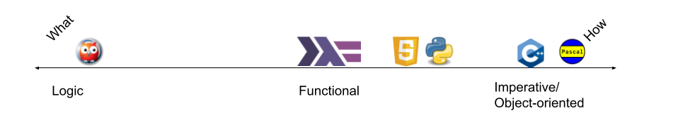
Prolog programs are made up of exactly three components:

Facts
Rules
Queries

The syntax of Prolog defines the rules for writing facts, rules and queries. Syntactic elements in Prolog belong to one of three categories:

Atoms: The most fundamental unit of a Prolog program. They are simply symbols. Usually they are simply sequences of characters that begin with a lowercase letter. However, atoms can contain spaces (in which case they are enclosed in ’s) and they can start with uppercase letters (in which case they are wrapped with ’s).
Variables: Like atoms, but variables always start with uppercase letters.
Functors: Like atoms, but functors define relationships/facts.

If Prolog is a logic programming language, there must be some means for specifying logical operations. There is! In the context of specifying a rule, the and operation is written using a ,. In the context of specifying a rule, the or operation is written using a ;. Obviously!

The best way to learn Prolog is to start writing some programs. We’ll come back to the theory later!

Just The Facts

At its most basic, a Prolog program is a set of facts:

takes(jane, cs4999).
takes(alicia, cs2020).
takes(alice, cs4000).
takes(mary, cs1021).
takes(bob, cs1021).
takes(kristi, cs4000).
takes(sam, cs1021).
takes(will, cs2080).
takes(alicia, cs3050).

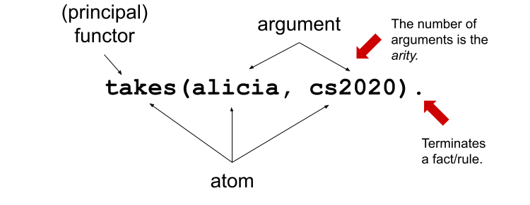
In relation to the first-order predicate logic that Prolog models, takes is a logical predicate. We’ll refer to them as facts or predicates, depending on what’s convenient. Formally, they predicates and facts are written as /. Two (or more) facts/predicates with the same functor but different arities are not the same. For instance, takes/1 and takes/2 are completely different.

Let’s read one of these facts in English:

takes(jane, cs4999).

could be read as “Jane takes CS4999.”. As programmers, we know what that means: the student named Jane is enrolled in the class CS4999. However, Prolog does not share our sense of meaning! Prolog simply thinks that we are defining one element of the takes relationship where jane is somehow related to cs4999. As a Prolog programmer, we could just has easily have written

tennis_shoes(jane, cs4999).
tennis_shoes(alicia, cs2020).
tennis_shoes(alice, cs4000).
tennis_shoes(mary, cs1021).
tennis_shoes(bob, cs1021).
tennis_shoes(kristi, cs4000).
tennis_shoes(sam, cs1021).
tennis_shoes(will, cs2080).
tennis_shoes(alicia, cs3050).

and gotten the same result! But, we programmers want to define something that is meaningful, so we choose to use atoms that reflect their semantic meaning. With nothing more than the facts that we have defined above, we can write queries. In order to interact with queries in real time, we can use the Prolog REPL. Once we have started the Prolog REPL, we will see a prompt like this:

?-

The world awaits …

To load a Prolog file in to the REPL, we will use the consult predicate:

?- consult('intro.pl').
true.

The Prolog facts, rules and queries in the intro.pl file are now available to us. Assume that intro.pl contains the takes facts from above. Let’s make some queries:

?- takes(bob, cs1021).
true.

?- takes(will, cs2080).
true.

?- takes(ali, cs4999).
false.

These are simple yes/no queries and Prolog obliges us with terse answers. But, even with the simple facts shown above, Prolog can be used to make some powerful inferences. Prolog can tell us the names of all the people it knows who are taking a particular class:

?- takes(Students, cs1021).
Students = mary ;
Students = bob ;
Students = sam.

Wow! Here Prolog is telling us that there are three different values of the Students variable that will make the query true: mary, bob and sam. In the lingo, Prolog is unifying Students with the values that will make our query true. Let’s go the other way around:

?- takes(alicia, Classes).
Classes = cs2020 ;
Classes = cs3050.

Here Prolog is telling us that there are two different classes that Alicia is taking. Nice.

That’s great, but pretty limited: it’s kind of terrible if we had to write out each fact explicitly! The good news is that we don’t have to do that! We can use a Prolog rule to define facts based on the existence of other facts. Let’s define a rule which will tell us the students who are CS majors. To be a CS major, you must be taking (exactly) two classes:

cs_major(X) :- takes(X, Y), takes(X, Z), Y @< Z.

That’s lots to take in at first glance. Start by looking at the general format of a rule:

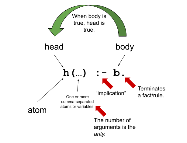
Okay, so now back to our particular rule that defines what it means to be a CS Major. (For the purposes of this discussion, assume that the @< operator is “not equal”). Building on what we know (e.g., , is and, :- is implication, etc), we can read the rule like: “X is a CS Major if X takes class Y and X takes class Z and class Y and Z are not the same class.” Pretty succinct definition.

To make the next few examples a little more meaningful, let’s update our list of facts before moving on:

takes(jane, cs4999).
takes(alicia, cs2020).
takes(alice, cs4000).
takes(mary, cs1021).
takes(bob, cs1021).
takes(bob, cs8000).
takes(kristi, cs4000).
takes(sam, cs1021).
takes(will, cs2080).
takes(alicia, cs3050).

With that, let’s find out if our rule works as intended!

?- cs_major(alicia).
true ;
false.

Wow! Pretty cool! Prolog used the rule that we wrote, combined it with the facts that it knows, and inferred that Alicia is a CS major! (For now, disregard the second False – we’ll come back to that!). Like we could use Prolog to generate the list of classes that a particular student is taking, can we ask Prolog to generate a list of all the CS majors that it knows?

?- cs_major(X).
X = alicia ;
X = bob ;
false.

Boom!

11/5/2021

*The retreat to move forward.

Backtracking

In today’s lecture, we discussed the concepts of backtracking and choice points in order to learn how Prolog can determine the meaning of our programs.

There is a formal definition of choice points and backtracking from the Prolog glossary:

backtracking: Search process used by Prolog. If a predicate offers multiple clauses to solve a goal, they are tried one-by-one until one succeeds. If a subsequent part of the proof is not satisfied with the resulting variable binding, it may ask for an alternative solution, causing Prolog to reject the previously chosen clause and try the next one.

There are lots of undefined words in that definition! Let’s dig a little deeper.

A predicate is like a boolean function. A predicate takes one or more arguments and yields true/false. As we said at the outset of our discussion about declarative programming languages, the reason that a predicate may yield true or false depends on the semantics imposed upon it from the outside. A predicate is a term borrowed from first-order logic, a topic that we will return to in later lectures.

Remember our takes example from previous lectures? takes is a predicate! takes has two arguments and returns a boolean.

In Prolog, rules and facts are written to define predicates. A rule defines the conditions under which a predicate is true using a body – a list of other predicates, logical conjunctives, implications, etc. See The Daily PL - 11/3/2021 for additional information about rules. A fact is a rule without a body and unconditionally defines that a certain relationship is true for a predicate.

related(will, bill).
related(ali, bill).
related(bill, william).

related(X, Y) :- related(X, Z), related(Z, Y).

In the example above, related is a predicate defined by facts and rules. The facts and rules above are the clauses of the predicate.

choicepoint: A choice point represents a choice in the search for a solution. Choice points are created if multiple clauses match a query or using disjunction (;/2). On backtracking, the execution state of the most recent choice point is restored and search continues with the next alternative (i.e., next clause or second branch of ;/2).

That’s a mouthful! I think that the best way to understand this is to look at backtracking in action and see where choice points exist.

Give and Take

Remember the takes predicate that we defined in the last class:

takes(jane, cs4999).
takes(alicia, cs2020).
takes(alice, cs4000).
takes(mary, cs1021).
takes(bob, cs1021).
takes(bob, cs8000).
takes(kristi, cs4000).
takes(sam, cs1021).
takes(will, cs2080).
takes(alicia, cs3050).

We subsequently defined a cs_major predicate:

cs_major(X) :- takes(X, Y), takes(X, Z), Y @< Z.

The cs_major predicate says that a student who takes two CS classes is a CS major. Let’s walk through how Prolog would respond to the following query:

cs_major(X).

To start, Prolog realizes that in order to satisfy our query, it has to at least satisfy the query

takes(X, Y).

So, Prolog starts there. In order to satisfy that query, it searches its knowledge base (its list of facts/rules that define predicates) from top to bottom. X and Y are variables and the first appropriate fact that it finds is

takes(jane, cs4999).

So, it unifies X with jane and Y with cs4999. Having satisfied that query, Prolog realizes that it must also satisfy the query:

takes(X, Z).

However, Prolog has already provisionally unified X with jane. So, Prolog really attempts to satisfy the query:

takes(jane, Z).

Great. For Prolog, attempting to satisfy this query is completely distinct from its attempt to satisfy the query takes(X, Y) which means that Prolog starts searching its knowledge base anew (again, from top to bottom!). The first appropriate fact that it finds that satisfies this query is

takes(jane, cs4999).

So, it unifies Z with cs4999. Having satisfied that query too, Prolog moves on to the third query:

Y @< Z.

Unfortunately, because X and Y are both unified to cs4999, Prolog fails to satisfy that query. In other words, Prolog realizes that its provisional unification of X with jane, Y with cs4999 and Z with cs4999 is not a way to satisfy our original query (cs_major(X)).

Does Prolog just give up? Absolutely not! It’s persistent. It backtracks! To where?

Well, according to the definition above, it backtracks to the most-recent choicepoint! In this case, the most recent choicepoint was its provisional unification of Z with cs4999. So, Prolog forgets about that attempt, and restarts the search of its knowledge base.

Where does it restart that search, though? This is important: It restarts its search where it left off. In other words, it starts at the first fact at takes(jane, cs4999). Because there are no other facts about classes that Jane takes, Prolog fails again, this time attempting to satisfy the query takes(jane, Z).

I ask again, does Prolog just give up? No, it backtracks again! This time it backtracks to its most-recent choicepoint. Now, that most recently choicepoint was its provisional unification of X with jane. Prolog forgets that attempt, and restarts the search of its knowledge base! Again, because this is the continuation of a previous search, Prolog begins where it left off in its top-to-bottom search of its knowledge base. The next fact that it see is

takes(alicia, cs2020)

So, Prolog provisionally unifies X with alicia and Y with cs2020. Having satisfied that query (for a second time!), Prolog realizes that it must also satisfy the query:

takes(X, Z).

However, Prolog has provisionally unified X with alicia. So, Prolog really attempts to satisfy the query:

takes(alicia, Z).

Great. For Prolog, attempting to satisfy this query is completely distinct from its attempt to satisfy the query takes(X, Y) and its previous attempt to satisfy the query takes(jane, Z). Therefore, Prolog starts searching its knowledge base anew (again, from top to bottom!). The first appropriate fact that it finds that satisfies this query is

takes(alicia, cs2020).

So, it unifies Z with cs2020. Having satisfied that query too, Prolog moves on to the third query:

Y @< Z.

Unfortunately, because Z and Y are both unified to cs2020, Prolog fails to satisfy that query. In other words, Prolog realizes that its provisional unification of X with alicia, Y with cs2020 and Z with cs2020 is not a way to satisfy our original query (cs_major(X)). Again, Prolog does not give up and it backtracks to its most recent choicepoint. The good news is that Prolog can satisfy the query

takes(alicia, Z)

a second way by unifying Z with cs3050. Prolog proceeds to the final part of the rule

X @< Y

which can be satisfied this time because cs3050 and cs2020 are different!

Victory!

Prolog was able to satisfy the original query when it unified X with alicia, Y with cs2020 and Z with cs3050.

Below is a visualization of the description given above:

A Prolog user at the REPL (or a Prolog program using this rule) could ask for all the ways that this query is satisfied. And, if the user/program does, then Prolog will backtrack as if it did not find a satisfactory unification for Z, Y or X (in that order!).* 11/5/2021

11/8/2021

In the true spirit of a picture being worth a thousand words , think of this Daily PL as a graphic novel.

Going Over Backtracking Again (see what I did there?)

In today’s lecture, we went deeper into the discussion of backtracking and saw its utility. In particular, we discussed the following Prolog program for generating all the integers.

generate_integer(0).
generate_integer(X) :- generate_integer(Y), X is Y + 1.

This is an incredibly succinct way to declare what it means to be an integer. This generator function is attributable to Programming in Prolog by Mellish and Clocksin (Links to an external site.). In other words, we know that it’s a reasonable definition.

As discussed in the description of Assignment 3, the best way to learn Prolog, I think, is to play with it! So, let’s see what this can do!

?- generate_integer(5).
true ;

In other words, it can be used to determine whether a given number is an integer. Awesome.

?- generate_integer(X).
X = 0 ;
X = 1 ;
X = 2 ;
X = 3 ;
X = 4 ;
X = 5 ;
X = 6

Woah, look at that … generate_integer/1 can do double duty and generate all the integers, too. Pretty cool!

The generation of the numbers using this definition is possible thanks to the power of backtracking. If you need a refresher on backtracking and/or choice points, I recommend previous Daily PLs.

The (im)possibility of using words to describe the backtracking involved in generate_integer/1, led me to create the following diagram that attempts to illustrate the process. I encourage you to look at the diagram, run generate_integer/1 in swipl with trace enabled and ask any questions that you have! Again, this is not a simple concept, but once you understand what is going on, Prolog will begin to make more sense!

It may be necessary to use a high-resolution version of the diagram if you are curious about the details. Such a version is available in SVG format here.

Chasing Our Tails

Yes, I can hear you! I know, generate_integer/1 is not tail recursive. We learned that tail recursion is a useful optimization in functional programming languages (and even imperative programming languages). Does that mean that it’s an important optimization in Prolog?

To find out, I timed how long it took Prolog to answer the query

?- generate_integer(50000).

The answer? On my desktop computer, it took 1 minute and 48 seconds.

If we want something for comparison, we’ll have to come up with a tail-recursive version of generate_integer/1. Let’s call it generate_integer_tr/1 (creative, I know), and define it like:

generate_integer_tr(X) :- next_integer(0,X).

next_integer(J, J).
next_integer(J, L) :- K is J + 1, next_integer(K, L).

The fact next_integer(J, J) is a “trick” to define a base case for our definition in the same way that generate_integer(0) was a base case in the definition of generate_integer/1. To get a sense for the need for next_integer(J, J) think about what happens when the first query of next_integer(0,X) is performed in order to satisfy the query generate_integer_tr(50000). In this case, the next_integer(J, J) fact matches (convince yourself why! Hint: there are no restrictions on J). As a result, J unifies with the 0, and the X unifies with the J. That’s great, but (X = ) 0 does not equal 50000. So, Prolog does what?

In unison: BACKTRACKS.

The choice point is Prolog’s selection of next_integer(J, J), so Prolog tries again at the next possible fact/rule: next_integer(J, L) :- K is J + 1, next_integer(K, L). J is unified with 0, K is unified with 1 (J + 1) and Prolog must now satisfy a new goal: next_integer(1, L). Because this query for next_integer/1 is completely different than the one it is currently attempting to satisfy, Prolog starts the search anew at the top of the list of facts. The first fact to match? next_integer(J, J). Therefore, J unifies with 1, L unifies with J (making L 1), and X (from the initial query) unifies with L. Unfortunately, the result again does not satisfy our query. But, Prolog persists and backtracks but only as far as the second attempt to satisfy next_integer (using next_integer(J,J)). In much the same way that generate_integer/1 worked, Prolog continues to progress, then backtrack, then progress, then backtrack … while solving the generate_integer_tr(50000) query.

The difference between the two functions is that in next_integer/2, the recursive act is the last thing that is done. In other words, generate_integer_tr/1 is tail recursive.

Does this impact performance? Absolutely! On my desktop. Prolog can answer the query generate_integer_tr(50000). in 0.029 seconds. Yeow!

11/10/2021

In today’s class we learned about a workhorse rule in logic programming: append/3. append/3 can be used to implement many other different rules, including a rule that will generate all the permutations of a list!

Pin the Tail on the List

The goal (pun intended) of append is to determine whether two lists, X and Y, are the same as a third list, Z, when appended together. We could use the append query like this:

?- append([1,2,3], [a,b,c], [1,2,3,a,b,c]).
true.

?- append([1,2,3], [a,b], [1,2,3,a,b,c]).
false.

What we will find is that append/3 has a hidden superpower besides its ability to simply answer yes/no queries like the ones above.

The definition of append/3 will follow the pattern of other recursively defined rules that we have seen so far. Let’s start with the base case. The result of appending an empty list with some list Y, is just list Y. Let’s write that down:

append([], Y, Y).

And now for the recursive case: appending list X to list Y yields some list Z where Z is the first element of the list X following by the result of appending the tail of X with Y. The natural language version of the definition is complicated but I think that the Prolog definition makes it more clear:

append([H|T], Y, [H|AppendedList]) :- append(T, Y, AppendedList).

Let’s see how Prolog attempts to answer the query append([1,2], [a,b], [1,2,a,b]).

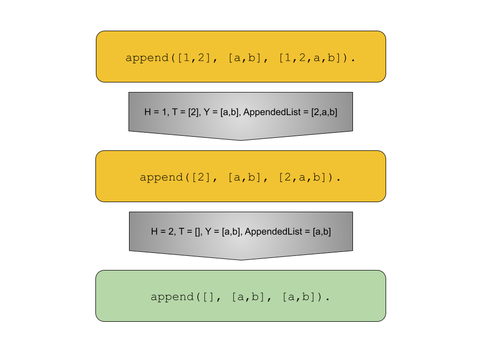
And now let’s look at it’s operation for the query append([1,2], [a,b], [1,a,b]).

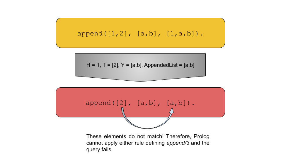
It’s also natural to look at append/3 as a tool to “assign” a variable to be the result of appending two lists:

?- append([1,2,3], [a,b,c], Z).
Z = [1, 2, 3, a, b, c].

Here we are asking Prolog to assign variable Z to be a list that holds the appended contents of the lists in the first two arguments.

Look at Append From a Different Angle

We’ve seen append/3 in action so far in a procedural way – answering whether two lists are equal to one another and “assigning” a variable to a list that holds the contents of another two lists appended to one another. But earlier I said that append/3 has some magical powers.

If we look at append/3 from a different angle, the declarative angle, we can see how it can be used to generate all the different combinations of two lists that, when appended together, yield a third list! For example,

?- append(X, Y, [1,2,3]).
X = [],
Y = [1, 2, 3] ;
X = [1],
Y = [2, 3] ;
X = [1, 2],
Y = [3] ;
X = [1, 2, 3],
Y = [] ;

Wow. That’s pretty cool! Prolog is telling us that it can figure out three different combinations of lists that, when appended together, will equal the list [1,2,3]. I mean, if that doesn’t make your blood boil, I don’t know what will.

Let’s Ride the Thoroughbred

The power of append/3 makes it useful in so many different ways. When I started learning Prolog, the resource I was using (Learn Prolog Now (Links to an external site.)) spent an inordinate amount of time discussing append/3 and it’s utility. It took me a long time to really understand the author’s point. A long time.

Prefix and Suffix

Let’s take a quick look at how to define a rule prefix/2. prefix/2 takes two arguments – a possible prefix, PP, and a list, L – and determines whether PP is a prefix of L. We’ve gotten so used to writing recursive definitions, it seems obvious that we would define prefix/2 using that pattern. In the base case, an empty list is a prefix of any list:

prefix([], _).

(Remember that _ is “I don’t care.”). With that out of the way, we can say that PP is a prefix of L if

the head element of PP is the same as the head element of L, and the tail of PP is a prefix of the tail of L:

prefix([H|Xs], [H|Ys]) :- prefix(Xs, Ys).

Fantastic. That’s a pretty easy definition and it works in all the ways that we would expect:

?- prefix([1,2], [1,2,3]).
true.

?- prefix([1,2], [2,3]).
false.

?- prefix(X, [1,2,3]).
X = [] ;
X = [1] ;
X = [1, 2] ;
X = [1, 2, 3] ;

But, what if there was a way that we could write the definition of prefix/2 more succinctly! Remember, programmers are lazy – the fewer keystrokes the better!

Think about this alternate definition of prefix: PP is a prefix of L, when there is a (possibly empty) list, W (short for “whatever”), such that PP appended with W is equal to L. Did you see the magic word? Appended! We have append/3, so let’s use it:

prefix(PP, L) :- append(PP, _, L).

(Note that we have replaced W from a natural-language definition with _ because we don’t care about it’s value!)

We could go through the same process of defining suffix/2 recursively, or we could cut to the chase and define it in terms of append/3. Let’s save ourselves some time: SS is a suffix of L, when there is a (possibly empty) list, W (short for “whatever”), such that W appended with SS is equal to L. Let’s codify that:

suffix(SS, L) :- append(_, SS, L).

But, does it work?

?- suffix_append([3,4], [1,2,3,4]).
true.

?- suffix_append([3,5], [1,2,3,4]).
false.

?- suffix_append(X, [1,2,3,4]).
X = [1, 2, 3, 4] ;
X = [2, 3, 4] ;
X = [3, 4] ;
X = [4] ;
X = [] ;

Permutations

We’re all friends here, aren’t we? Good. I have no problem admitting that I am terrible at thinking about permutations of a set. I have tried and tried and tried to understand the section in Volume 4 of Knuth’s TAOCP (Links to an external site.) about generating permutations (Links to an external site.) but it’s just too hard for me. Instead, I just play around with them until I grok it. To help me play, I want Prolog’s help. I want Prolog to generate for me all the permutations of a given list. We will call this permute/2. Procedurally, permute/2 will say whether its second argument is a permutation of its first argument. Declaratively, permute/2 will generate a list of permutations of elements in the list in its first argument. Let’s work back from the end: We’ll see how it should work before actually defining it:

?- permutation([1,2,3], [3,1,2]).
true .

?- permutation([1,2,3], L).
L = [1, 2, 3] ;
L = [1, 3, 2] ;
L = [2, 1, 3] ;
L = [2, 3, 1] ;
L = [3, 1, 2] ;
L = [3, 2, 1] ;
false.

Cool. If I run permute/2 enough times I might start to understand them!

Now that we know the results of invoking permute/2, how are we going to define it? Again, let’s take the easy way out and see the definition and then walk through it piece-by-piece in order to understand its meaning:

permute([], []).
permute(List, [X|Xs]) :- append(W, [X|U], List), append(W, U, ListWithoutX), permute(ListWithoutX, Xs).

Well, the first rule is simple – the permutation of an empty list is just the empty list!

The second rule, well, not so much! There are three conditions that must be satisfied for a list defined as [X|Xs] to be a permutation of List.

Think of the first condition in a declarative sense: “Prolog, make me two lists that, when appended together, equal List. Name the first one W. And, while you’re at it, make sure that the first element in the second list is X and call the tail of the second list U. Thanks.”

Think of the second condition in a procedural sense: “Prolog, append W and U to create a new list named ListWithoutX.” The name ListWithoutX is pretty evocative because, well, it is a list that contains every element of List but X.

Finally, think of the third condition in a declarative sense: “I want Xs to be all the possible permutations of ListWithoutX – Prolog, make it so!”

Let’s try to put all this together into a succinct natural-language definition: A list whose first element is X and whose tail is Xs is a permutation of List if:

X is one of the elements of List, and
Xs is a permutation of the list List without element X.

Below is a visualization of the process Prolog takes to generate the first two permutations of [1,2,3]:

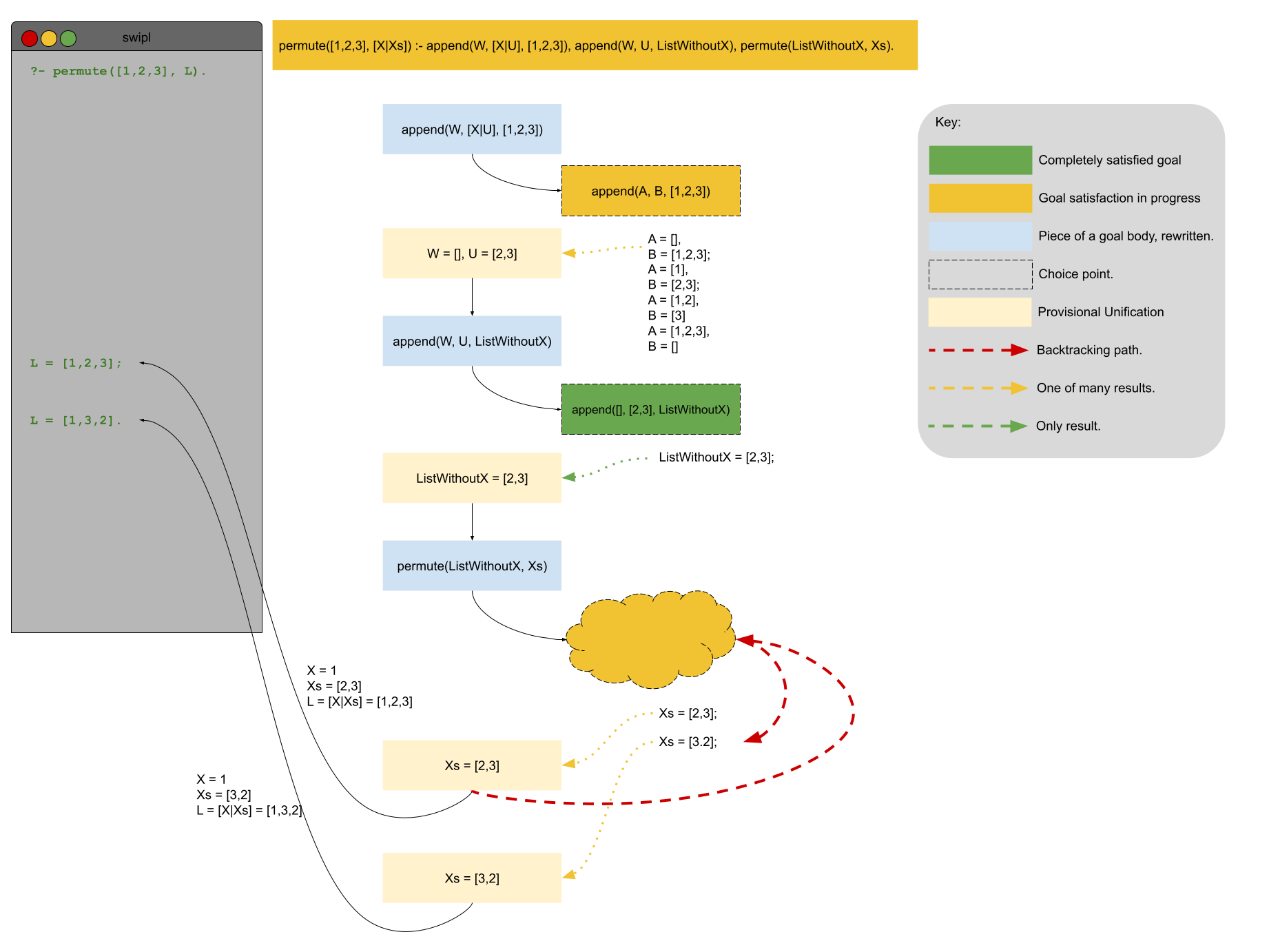
11/12/2021

If the append/3 predicate that we wrote on Wednesday is a horse that we can ride to accomplish many different tasks, then Prolog is like a wild stallion that tends to run in a direction of its choosing. We can use cuts to tame our mustang and make it go where we want it to go!

The Possibilities Are Endless

Let’s start the discussion by writing a merge/3 predicate. The first two arguments are sorted lists. The final argument should unify to the in-order version of the first two arguments merged. Before starting to write some Prolog, let’s think about how we could do this.

Let’s deal with the base cases first: When either of the first two lists are empty, the merged list is the non-empty list. We’ll write that like

merge(Xs, [], Xs).
merge([], Ys, Ys).

And now, for the recursive cases: We will call the first argument Left, the second argument Right, and the third argument Sorted. The first element of Left can be called HeadLeft and the rest of Left can be called TailLeft. The first element of Right can be called HeadRight and the rest of Right can be called TailRight. In order to merge, there are three cases to consider:

HeadLeft is less than HeadRight
HeadLeft is equal to HeadRight
HeadRight is less than HeadLeft

For case (1), the head of the merged result is HeadLeft and the tail of the merged result is the result of merging TailLeft with Right. For case (2), the head of the merged result is HeadLeft and the tail of the merged result is the result of merging TailLeft with TailRight. For case (3), the head of the merged result is HeadRight and the tail of the merged result is the result of merging Left with TailRight.

It’s far easier to write this in Prolog than English:

merge([X|Xs], [Y|Ys], [X|Zs]) :- X<Y, merge(Xs, [Y|Ys], Zs).
merge([X|Xs], [Y|Ys], [X|Zs]) :- X=:=Y, merge(Xs, Ys, Zs).
merge([X|Xs], [Y|Ys], [Y|Zs]) :- Y<X, merge([X|Xs], Ys, Zs).

(Note: : is the “equal to” boolean operator in Prolog. See =:=/2 (Links to an external site.) for more information.

For merge/3, let’s write the base cases after our recursive cases. With that switcheroo, we have the following complete definition of merge/3:

merge([X|Xs], [Y|Ys], [X|Zs]) :- X<Y, merge(Xs, [Y|Ys], Zs).
merge([X|Xs], [Y|Ys], [X|Zs]) :- X=:=Y, merge(Xs, Ys, Zs).
merge([X|Xs], [Y|Ys], [Y|Zs]) :- Y<X, merge([X|Xs], Ys, Zs).
merge(Xs, [], Xs).
merge([], Ys, Ys).

Let’s follow Prolog as it attempts to use our predicate to answer the query

merge([1, 3, 5], [2,4,6], M).

As we know, Prolog will search top to bottom when looking for ways to unify and the first rule that Prolog sees is applicable:

merge([X|Xs], [Y|Ys], [X|Zs]) :- X<Y, merge(Xs, [Y|Ys], Zs).

Why? Because Prolog sees X as 1 and Y as 2 and 1 < 2. Therefore, Prolog will complete its unification for this query by replacing it with another query:

merge([3,5], [2,4,6], Zs).

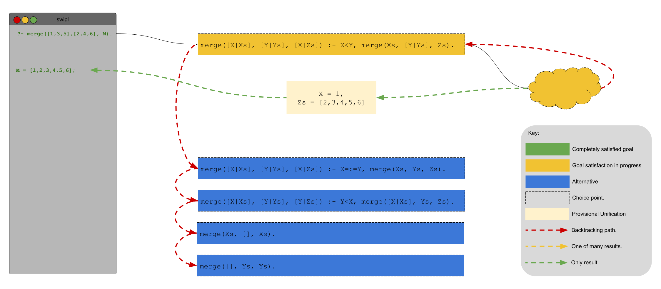
Once Prolog has completed that query, the response comes back:

M = [1,2,3,4,5,6]

Unfortunately, that’s not the whole story. While Prolog is off attempting to satisfy the subquery merge([3,5], [2,4,6], Zs)., it believes that there are still several other viable alternatives for satisfying our original query:

merge([X|Xs], [Y|Ys], [X|Zs]) :- X=:=Y, merge(Xs, Ys, Zs).
merge([X|Xs], [Y|Ys], [Y|Zs]) :- Y<X, merge([X|Xs], Ys, Zs).
merge(Xs, [], Xs).
merge([], Ys, Ys).

The result is that Prolog will have to use memory to remember those alternatives. As the lists that we ask Prolog to merge get longer and longer, that memory will have an impact on the system’s performance. However, we know that those other alternatives will never match and keeping them around is a waste. How do we know that? Well, if X < Y then it cannot be equal to Y and it certainly cannot be greater than Y. Moreover, the lists in the first two arguments cannot be empty. Overall, each of the possible rules for merge/3 are mutually exclusive. You can only choose one.

If there were a way to tell Prolog that those other possibilities are impossible after it encounters a matching rule that would save Prolog from having to keep them around. The good news is that there is!

We can use the cut (Links to an external site.) operator to tell Prolog that once it has “descended” down a particular path, there is no sense backtracking beyond that point to look for alternate solutions. The technical definition of a cut is

Discard all choice points created since entering the predicate in which the cut appears. In other words, commit to the clause in which the cut appears and discard choice points that have been created by goals to the left of the cut in the current clause.

Let’s rewrite our merge/3 predicate to take advantage of cuts and save some overhead:

merge([X|Xs], [Y|Ys], [X|Zs]) :- X<Y, !, merge(Xs, [Y|Ys], Zs).
merge([X|Xs], [Y|Ys], [X|Zs]) :- X=:=Y, !, merge(Xs, Ys, Zs).
merge([X|Xs], [Y|Ys], [Y|Zs]) :- Y<X, !, merge([X|Xs], Ys, Zs).
merge(Xs, [], Xs) :- !.
merge([], Ys, Ys) :- !.

Returning to the definition of cut, in the first rule we are telling Prolog (through our use of the cut) to disregard all choice points created to the left of the !. In particular, we are telling Prolog to forget about the choice it made that X < Y. The result is that Prolog is no longer under the impression that there are other rules that are applicable. Visually, the situation resembles

Merge Cut.png

Dr. Cutyll and Mr. Unify

Cuts are not always so beneficial. In fact, their use in Prolog is somewhat controversial. A cut necessarily limits Prolog’s ability to backtrack. If the Prolog programmer uses a cut in a rule that is meant to be used declaratively (in order to generate values) and procedurally, then the cut may change the results.

There are two types of cuts. A green cut is a cut that does not change the meaning of a predicate. The cut that we added in the merge/3 predicate above is a green cut. A red cut is, technically speaking, a cut that is not a green cut. I know that’s a satisfying definition. Sorry. The implication, however, is that a red cut is a cut that changes the meaning of predicate.

11/15/2021

Red Alert

At the end of lecture on Friday, we discussed the two different types of cuts – red and green. A green cut is one that does not alter the behavior of a Prolog program. A red cut does alter the behavior of a Prolog program. The implication was that red cuts are bad and green cuts are good. But, is this always the case?

To frame our discussion, let’s look at a Prolog program that performs a Bubble Sort on a list of numbers. The predicate, bsort/2, is defined like this:

bsort(Unsorted, Sorted):-
  append(Left, [A, B | Right], Unsorted),
  B<A,
  append(Left, [B, A | Right], MoreSorted),
  bsort(MoreSorted, Sorted).
bsort(Sorted, Sorted).

The first rule handles the recursive case (when there is at least one list item out of order) and the second rule handles the base case (when the list is sorted). According to this definition, how does Prolog handle the query

bsort([2,1,3,5], M).

Prolog (as we are well aware) searches its rule top to bottom. The first rule that it sees is the recursive case and Prolog immediately opts for it. Opting for this case is not without consequences – a choice point is created. Why? Because Prolog made the choice to attempt to satisfy the query according to the first rule and not the (just as applicable) second rule! Let’s call this choice point A.

Next, Prolog attempts to unify the subquery append(Left, [A, B | Right], Unsorted). The first (of many) unifications that append/3 generates is Left = [], A = 2, B = 1, Right = [3, 5]. By continuing with this particular unification, Prolog creates another choice point. For what reason? Well, Prolog knows that append/3 could generate other potential unifications and it will need to check those to see if they, too, satisfy the original query! Let’s call this choice point B. Next, Prolog checks whether A is less than B – it is. Prolog continues in a like manner to satisfy the final two subgoals of the rule.

When Prolog does satisfy those, it has generated a sorted version of [2,1,3,5]. It reports that result to the querier. Great! There’s only one problem. There are still choice points that Prolog wants to explore. In particular, there are choice points A and B. In this case, we can forget about choice point B because there are no other unifications of append/3 that meet the criteria for A<B in Unsorted. In other words, visually the situation looks like this:

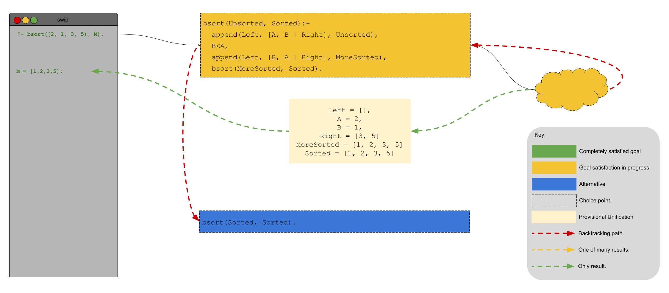
If the querier is using bsort/2 declaratively, this scenario is a problem: Prolog will backtrack to choice point A and then consider the base case rule for bsort/2. In other words, Prolog will also generate

[2,1,3,5]

as a unification! This is clearly not right. What’s more, the Prolog programmer could query for

bsort([3,2,1,4,5], Sorted).

in which choice point B will have consequences. Run this query for yourself (using trace), examine the results, and make sure you understand why the results are generated.

So, what are we to do? cut/0 (Links to an external site.) to the rescue! Logically speaking, once our bsort/3 rule finds a single element out of order and we adjust that element, the recursive call to itself will handle ordering any other unordered elements. In other words, we can forget any earlier choice points! This is exactly what the cut is intended for!

Let’s rewrite bsort/3 using cuts and see if our problem is sorted (see what I did there?):

bsort(Unsorted, Sorted):-
  append(Left, [A, B | Right], Unsorted),
  B<A, !,
  append(Left, [B, A | Right], MoreSorted),
  bsort(MoreSorted, Sorted).
bsort(Sorted, Sorted).

And now let’s see how our earlier troublesome queries perform:

?- bsort([2,1,3,5], Sorted).
Sorted = [1, 2, 3, 5].

?- bsort([3,2,1,4,5], Sorted).
Sorted = [1, 2, 3, 4, 5].

Amazing!

Here’s the rub: The version of our Prolog program with the cut gave different results than the version without. Is this cut a green or a red cut? That’s right, it’s a red cut. I guess there are such things as good red cuts after all!

The Fundamentals

As we have said in the past, there is a theoretical underpinning for each of the programming paradigms that we have studied this semester. Logic programming is no different. The theory behind logic programming is first-order predicate logic. Predicate logic is an extension of propositional logic. Propositional logic is based on the evaluation of propositions.

A proposition is simply any statement that can be true or false. For example,

Will is a programmer.
Alicia is a programmer.
Sam is a programmer.

Those statements can be true or false. In propositional logic we can build more complicated propositions from existing propositions using logical connectives like and, or, not, and implication (if … then). Each of these has an associated truth table to determine the truth of two combined propositions.

Look closely at the example propositions above and you will notice an underlying theme: they all do with someone (let’s call them x) being a programmer. In propositional logic, our ability to reason using that underlying theme is impossible. We can only work with the truth of the statement as a whole.

If we add to propositional logic variables, constants, and quantifiers then we get predicate logic and we are able to reason more subtly. Although you might argue that propositional logic has variables, everyone can agree that they are limited – they can only have two values, true and false. In first-order predicate logic, variables can have domains other than just {T, F}. That’s already a huge step!

Quantifiers “define” variables and “constrain” their possible values. There are two quantifiers in first-order predicate logic – the universal and the existential. The universal is the “for all” (aka “every”) quantifier. We can use the universal quantifier to write statements (in logic) like “Every person is a Bearcats fan.” Symbolically, we write the universal quantifier with the \(\forall\). We can write our obvious statement from above in logic like

\(\forall x(person(x) \Longrightarrow fan(x, bearcats))\)

Now we are talking! As for the existential quantifier, it allows us to write statements (in logic) like “There is some person on earth that speaks Russian.” Symbolically, we write the existential quantifier with the \(\exists\). We can write the statement about our Russian-speaking person as

\(\exists x(person(x) \land speaks(x, russion))\)

How are quantifiers embedded in Prolog? Variables in Prolog queries are existentially qualified – “Does there exist …?“ Variables in Prolog rules are universally quantified – “For all ….”

In first-order predicate logic, there are such things as Boolean-valued functions. This is familiar territory for us programmers. A Boolean-valued function is a function that has 0 or more parameters and returns true or false.

With these definitions, we can now define predicates: A predicate is a proposition in which some Boolean variables are replaced by Boolean-valued functions and quantified expressions. Let’s look at an example.

\(p \Longrightarrow q\)

is a proposition where p and q are boolean variables. Replace p with the Boolean-valued function \(is\_teacher(x)\) and q with the quantified expression \(\exists y(student(x) \land teaches(x, russion))\) and we have the predicate

\(is\_teacher(x) \Longrightarrow \exists y(student(x) \land teaches(x,y))\)

There is only one remaining question: Why is it called first-order predicate logic and not, say, higher-order predicate logic? “First-order” here indicates that the predicates in this logic cannot manipulate or reason about predicates themselves. Does this sound familiar? Imperative languages can define functions but they cannot reason about functions themselves while functional languages can!

11/17/2021

So far in this course we have covered lots of material. We’ve learned lots of definitions, explored lots of concepts and programmed in languages that we’ve never seen before. In all that time, though, we never really got to the bottom of one thing: What exactly is a language? In the final module of this course, we are going to cover exactly that!

Back to Basics

Let’s think way back to August 23 and recall two very important definitions: syntax and semantics. On that day we defined semantics as the effect of each statement’s execution on the program’s operation. We defined syntax as the rules for constructing structurally valid (note: valid, not correct) computer programs in a particular language. There’s that word again – language.

Before starting to define language, let me offer you two alternate definitions for syntax and semantics that draw out the distinction between the two:

The syntax of a programming language specifies the form of its expressions, statements and program units.
The semantics of a programming language specifies the meaning of its expressions, statements and program units.

It is interesting to see those two definitions side-by-side and realize that they are basically identical with the exception of a single word! One final note about the connection between syntax and semantics before moving forward: Remember how a well-designed programming language has a syntax that is evocative of meaning. In other words, a well-designed language might allow variables to contain a symbol like ? which would allow the programmer to indicate that it holds a Boolean.

Before we can specify a syntax for a programming language, we need to specify the language itself. In order to do that, we need to start by defining the language’s alphabet – finite set of characters that can be used to write sentences in that language. We usually denote the alphabet of a language with the \(\sum\). It is sometimes helpful to denote the set of all the possible sentences that can be written using the characters in the alphabet. We usually denote that with \(\sum\). For example, say that \(sum = \{a, b\}\), then \(\sum = \{a, b, aa, ab, ba, aaa, aab, aba, abb, …\}\). Notice that even though \(|\sum|\) is finite (that is, the number of elements in is finite), \(|\sum| = \infty\).

The alphabet of the C++ programming language is large, but it’s not infinite. However, the set of sentences that can be written using that alphabet is. But, as we all learn early in our programming career, just because you can write out a program using the valid symbols in the C++ alphabet does not mean the program is syntactically valid. The very job of the compiler is to distinguish between valid and invalid programs, right?

Let’s call the language that we are defining \(L\) and say that it’s alphabet is \(\sum\). \(L\) can be thought of as the set of all valid sentences in the language. Therefore, every sentence that is in \(L\) is in \(\sum\) – \(L \subseteq \sum\).

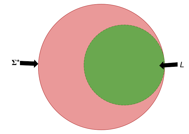
Look closely at the relationship between \(\sum\) and \(L\). While \(L\) never includes a sentence that is not included in \(\sum\), they can be identical! Think of some languages where any combination of characters from its alphabet are valid sentences! Can you come up with one?

The Really Bad Programmer

So, how can we determine whether a sentence made up of characters from the alphabet is in the language or not? We have to be able to answer this question – one of the fundamental jobs of the compiler, after all, is to do exactly that. Why not just write down every single valid sentence in a giant chart and compare the program with that list? If the program is in the list, then it’s a valid program! That’s easy.

Not so fast. Aren’t there an infinite number of valid C++ programs?

int main() {
  if (true) {
    if (true) {
      if (true) {
        ...
          std::cout << "Hello, World.";
      }
    }
  }
}

Well, dang. There goes that idea.

I guess we need a concise way to specify how to describe sentences that are in the language and those that are not. Before we start to think about ways to do that, let’s think back to Prolog. One of the really neat things about Prolog was the ability to specify something that had, at the same time, an ability to recognize and generate valid solutions to a set of constraints. Even in our simplest Prolog example, we could write down a set of facts and the language could determine whether a student took a particular class (giving us a yes/no answer) or generate a list of the people who were taking a particular class!

It would be great to have a tool that does the same thing for languages – a common description that allows us to create something that recognizes and generates valid sentences in the language. We will do exactly that!

Language Classes

The famous linguist Noam Chomsky was the first to recognize how there is a hierarchy of languages. The hierarchy is founded upon the concept of how easy/hard it is to write a concise definition for the language’s valid sentences.

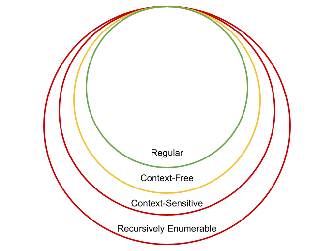
Each level of Chomsky’s Hierarchy, as it is called, contains the levels that come before it. Which languages belong to which level of the hierarchy is something that you will cover more in CS4040. (Note: The languages that belong to the Regular level can be specified by regular expressions (Links to an external site.). Something I know some of you have written before!)

For our purposes, we are going to be concerned with those languages that belong to the Context-Free level of the hierarchy.

Context-Free Grammars

The tool that we can use to concisely specify a Context-Free language is called a Context-Free Grammar. Precisely, a Context-Free Grammar, , is a set of productions , a set of terminal symbols, , a set of non-terminal symbols, , one of which is named

and is known as the start symbol.

That’s a ton to take in. The fact of the matter, however, is that the vocabulary is intuitive once you see and use a grammar. So, let’s do that. We will define a grammar for listing/recognizing all the positive integers:

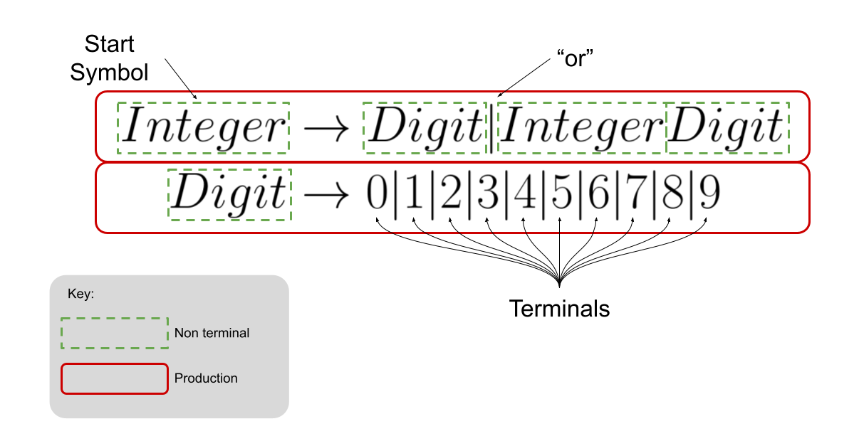
Now that we see an example of a grammar and its parts and pieces, let’s “read” it to help us understand what it means. Every valid integer in the language can be derived by writing down the start symbol and iteratively replacing every non-terminal according to a production until there are only terminals remaining! Again, that sounds complicated, but it’s really not. Let’s look at the derivation for the integer 142:

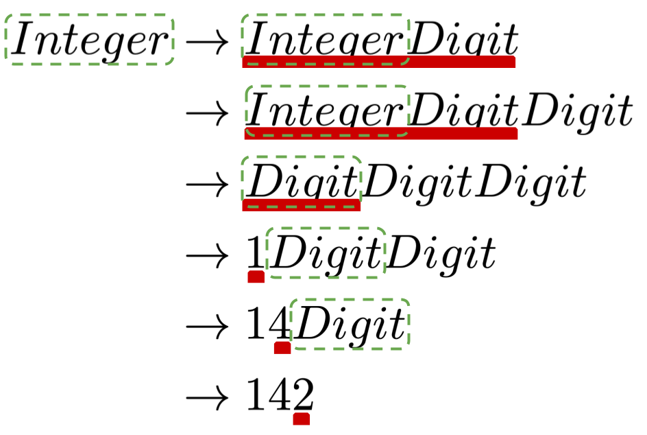
We start with the start symbol Integer and use the first production to replace it with one of the two options in the production. We choose to use the second part of the production and replace Integer with Integer Digit. Next, we use a production to replace Integer with Integer Digit again. At this point we have Integer Digit Digit. Next, we use one of the productions to replace Integer with Digit and we are left with Digit Digit Digit. Our next move is to replace the left-most Digit non-terminal with a terminal – the 1. We are left with 1 Digit Digit. Pressing forward, we replace the left-most Digit with 4 and we come to 14Digit. Almost there. Let’s replace Digit with 2 and we get 142. Because 142 contains only terminals, we have completed the derivation. Because we can derive 142 from the grammar, we can confidently say that 142 is in the language described by the grammar.

11/19/2021

(Context-free) Grammars (CFG) are a mathematical description of a language-generation mechanism. Every grammar defines a language. The strings in that language are those that can be derived from the grammar’s start symbol. Put another way, a CFG describes a process by which all the sentences in a language can be enumerated, or generated.

Defining a way to generate all the sentences in a grammar is one way to specify a language. Another way to define a language is to build a tool that separates sentences that are in the language from sentences that are not in the language. This tool is known as a recognizer. There is a relationship between recognizers and generators and we will explore that in future lectures.

Grammatical Errors

On Wednesday we worked with a grammar that purported to describe all the strings that looked like integers:

We performed a derivation using its productions to prove (by construction) that 142 is in the language. But, let’s consider this derivation:

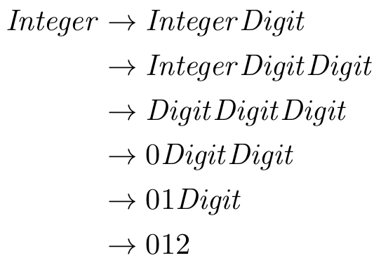
We have just proven (again, by construction) that 012 is an integer. This seems funny. A number that starts with 0 (that is not just a 0) should not be deemed an integer. Let’s see how we can fix this problem.

In order to guarantee that we cannot derive a number that starts with a 0 and deem it an integer, we will need to add a few more productions. First, let’s reconsider the production for the start symbol Integer. At the very highest level, we know that 0 is an integer. So, our start symbol’s production should handle that case.

With the base case accounted for, we next consider that an integer cannot start with a zero, but it can start with any other digit between 1 and 9. It seems handy to have a production for a non-terminal that expands to the terminals 1 through 9. We will call that non-terminal Nzd for non-zero digits. After the initial non-zero digit, an integer can contain zero or more digits between 0 and 9 (we can call this the rest of the integer). For brevity, we probably want a production that will expand to all the digits between 0 and 9. Let’s call that non-terminal Zd for zero digits. We’ll define it either as a 0 or anything in Nzd. If we put all of this together, we get the following grammar:

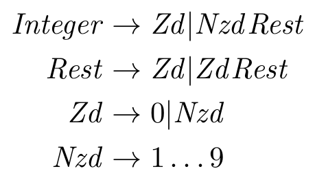
Let’s look at a few derivations to see if this gets the job done. Is 0 an integer?

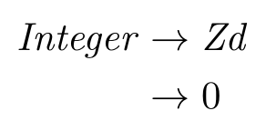
And a single-digit integer?

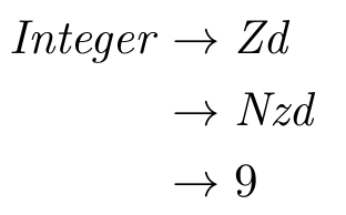
How about an integer between 10 and 100, inclusive?

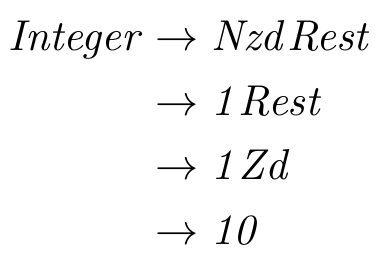
We are really cooking. Let’s try one more. Is a number greater than 100 derivable?

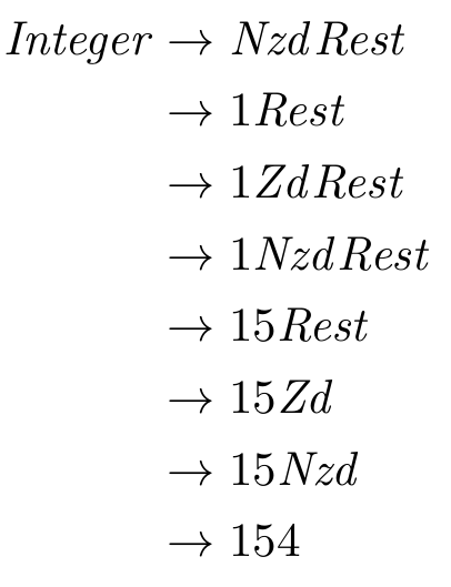
Think about this grammar and see if you can see any problems with it. Are there integers that cannot be derived? Are there sentences that can be derived that are not integers?

Trees or Derivations

Let’s take a look at a grammar that will generate sentences that are simple mathematical expressions using the + and * operators and the numbers 0 through 9:

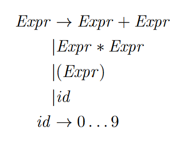
Until now we have used proof-by-construction through derivations to show that a particular string is in the language described by a particular grammar. What’s really cool is that any derivation can also be written in the form of a tree. The two representations contain the same information – a proof that a particular sentence is in a language. Let’s look at the derivation of the expression 1 + 5 * 2:

There’s only one problem with this derivation: Our choice of which production to apply to expand the start symbol was arbitrary. We could have just as easily used the second production and derived the expression 1 + 5 * 2:

This is clearly not a good thing. We do not want our choice of productions to be arbitrary. Why? When the choice of the production to expand is arbitrary, we cannot “encode” in the grammar any semantic meaning. (We will learn how to encode that semantic meaning below). A grammar that produces two or more valid parse trees for a particular sentence is known as an ambiguous grammar.

Let Me Be Clear

The good news is that we can rewrite the ambiguous grammar for mathematical expressions from above and get an unambiguous grammar. Like the way that we rewrote the grammar for integers, rewriting this grammar will involve adding additional productions:

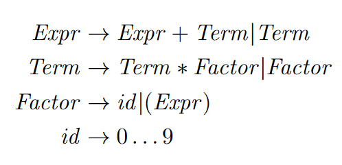
Using this grammar we have the following parse tree for the expression 1 + 5 * 2:

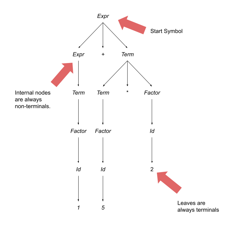
Before we think about how to encode semantic meaning in to a parse tree, let’s talk about the properties of a parse tree. The root node of the parse tree is always the start symbol of the grammar. The internal nodes of a parse tree are always non-terminals. The leaves of a parse tree are always terminals.

Making Meaning

If we adopt a convention that reading a parse tree occurs through a depth-first in-order traversal, we can add meaning to these beasts and their associated grammars. First, we can see how associativity is encoded: By writing all the productions so that “recursion” happens on the left side of any terminals (a so-called left-recursive production), we will arrive at a grammar that is left-associative. The converse is true – the productions whose recursion happens on the right side of any terminals (a right-recursive production) specifies right associativity. Second, we can see how precedence is encoded: The further away a production is from the start symbol, the higher the precedence. In other words, the precedence is inversely related to the distance from the start symbol. All alternate options for the same production have equal precedence.

Let’s look back at our grammar for Expr. A Term and an addition operation have the same precedence. A Factor and a multiplication operation have the same precedence. The production for an addition operation is left-recursive and, therefore, the grammar specifies that addition is left associative. The same is true for the multiplication operation.

11/22/2021

Before reading this Daily PL, please re-read the one from Friday, 11/19/2021. The content has been updated since it was originally published to reflect certain errors with the “better” Integer grammar we developed in class. Thanks, especially, to Jeroen for making sure that I got the grammar correct!

Making Meaning

In an earlier part of the class we talked about how to describe the dynamic semantics of a program. We worked closely with operational semantics but saw other examples, too (axiomatic and denotational). Although we said that what we are studying in this module is the syntax of a language and not its semantics, a language may have static semantics that the compiler can check during syntax analysis. Syntax analysis is done using a tool known as the parser.

Remember that syntax and syntax analysis is only concerned with valid programs. If the program, considered as a string of letters of the language’s alphabet, can be derived from the language grammar’s start symbol, then the program is valid. We all agreed that was the limit of what a syntax analyzer could determine.

One form of output of a parser is a parse tree. It is possible to apply “decoration” to the parse tree in order to verify certain extra-syntactic properties of a program at the time that it is being parsed. These properties are known as a language’s static semantics. More formally, Sebesta defines static semantics as the rules for a valid program in a particular language that are difficult (or impossible!) to encode in a grammar. Checking static semantics early in the compilation process is incredibly helpful for programmers as they write their code and allows the stages of the compilation process after syntax analysis to make more sophisticated assumptions about a program’s validity.

One example of static semantics of a programming language has to do with its type system. Checking a program for type safety is possible at the time of syntax analysis using an attribute grammar. An attribute grammar is an extension of a CFG that adds (semantic) information to its terminals and nonterminals. This information is known as attributes. Attached to each production are attribute calculation functions. At the time the program is parsed, the attribute calculation functions are evaluated every time that the associated production is used in a derivation and the results of that invocation are stored in the nodes of the parse tree that represent terminals and nonterminals. Additionally, in an attribute grammar, each production can have a set of predicates. Predicates are simply Boolean-valued functions. When a parser attempts to use a production during parsing, it’s not just the attribute calculation functions that are invoked – the production’s predicates are too. If any of those predicates returns false, then the derivation fails. An Assignment Grammar

To start class, we looked at a snippet of an industrial-strength grammar – the one for the C programming language. The snippet we saw concerned the assignment expression:

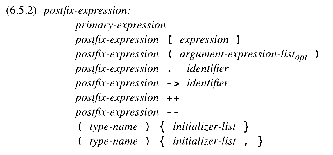
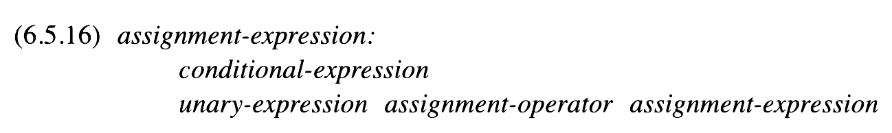
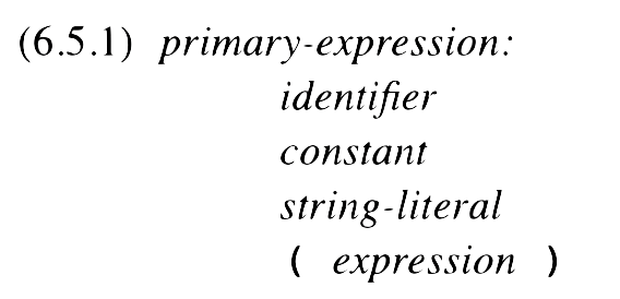
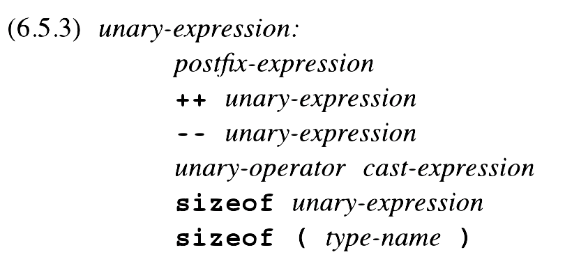
There are lots of details in the grammar for an assignment statement in C and not all of them pertain to our discussion. So, instead of using that grammar of assignment statements, we’ll use a simpler one:

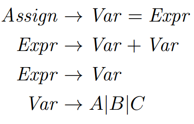
Assume that this is part of a larger grammar for a complete, statically typed programming language. In the subset of the grammar that we are going to work with, there are three terminals: A, B and C. These are variable names available for the programmer in our language. As a program in this language is parsed, the compiler builds a mapping between variables and their types (known as the symbol table), adding an entry for each new variable declaration it encounters. The compiler can “lookup” the type of a variable using its name thanks to the lookup function.

Our hypothetical language contains only two numerical types: int and real. A variable can only be assigned the result of an expression if that expression has the same type as the variable. In order to determine the type of an expression, our language adheres to the following rules:

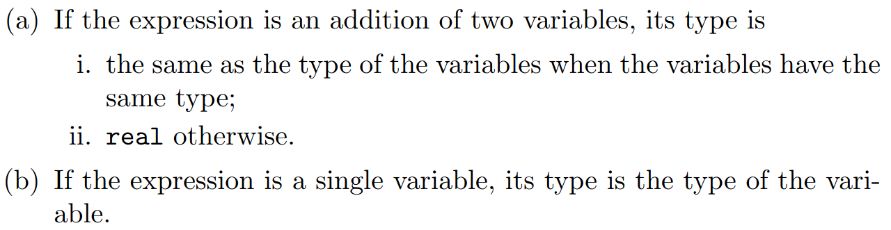
Let’s assume that we are looking at the following program written in our hypothetical language:

int A;
real B;
A = A + B;

The declarations of the variables A and B are handled by parts of the grammar that we are not showing in our example. Again, when those declarations are parsed, an entry is made in the symbol table so that variable names can be mapped to types. Let’s derive A = A + B; using the snippet of the grammar shown above:

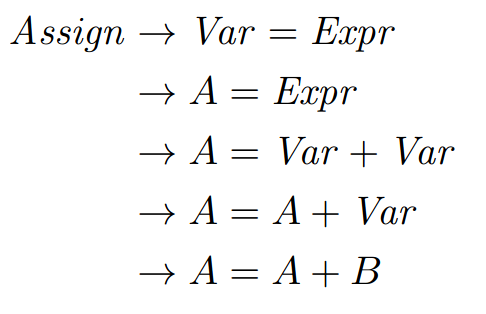
Great! The program passes the syntactic analysis so it’s valid!

Right?

This Grammar Goes To 11

Wrong. According to the language’s type rules, we can only assign to variables that have the same type as the expression being assigned. The rules say that A + B is a real (a.ii). A is declared as an int. So, even though the program parses, it is invalid!

We can solve this using attribute grammars and that’s exactly what we are going to do! For our Assign grammar, we will add the following attributes to each of the terminals and nonterminals:

expected_type: The type that is expected for the expression. actual_type: The actual type of the expression.

The values for the attributes are set according to functions. An attribute whose calculation function uses attribute values from only its children and peer nodes in the parse tree is known as a synthesized attribute. An attribute whose calculation function uses only attribute values from its parent nodes in the parse tree is known as an inherited attribute.

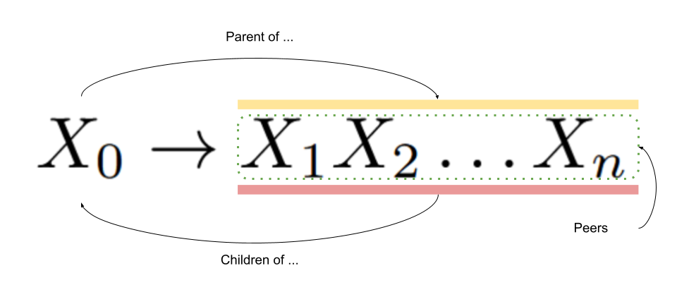
Let’s define the attribute calculation functions for the expected_type and actual_type attributes of the Assign grammar:

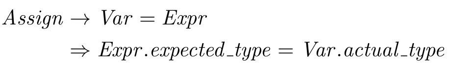
For this production, we can see that the expression’s expected_type attribute is defined according to the variable’s actual_type which means that it is an inherited attribute.

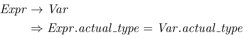
For this production, we can see that the expression’s actual_type attribute is defined according to the variable’s actual_type which means that it is a synthesized attribute.

And now for the most complicated (but not complex) attribute calculation function definition:

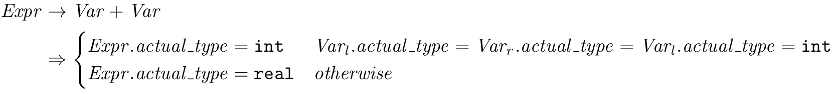
Again, we can see that the expression’s actual_type attribute is defined according to its children nodes – the actual_type of the two variables being added together – which means that it is a synthesized attribute.

If you are thinking that the attribute calculation functions are recursive, you are exactly right! And, you can probably see a problem straight ahead. So far the attribute calculation functions have relied on attributes of peer, children and parent nodes in the parse tree to already have values. Where is our base case?

Great question. There’s a third type of attribute known as an intrinsic attribute. An intrinsic attribute is one whose value is calculated according to some information outside the parse tree. In our case, the actual_type attribute of a variable is calculated according to the mapping stored in the symbol table and accessible by the lookup function that we defined above.

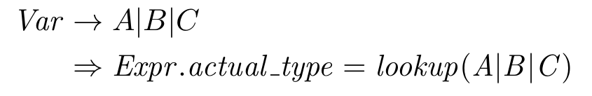
That’s all for the definition of the attribute calculation functions and is all well and good. Unfortunately, we still have not used our attributes to inform the parser when a derivation has gone off the rails by violating the type rules. We’ll define these guardrails predicate functions and show the complete attribute grammar at the same time:

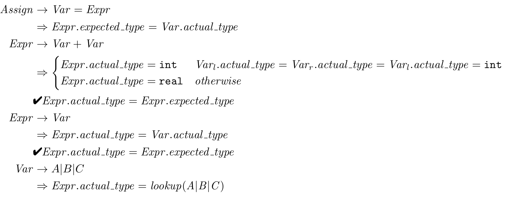
The equalities after the checkmarks are the predicates. We can read them as “If the actual type of the expression is the same as the expected type of the predicate, then the derivation (parse) can continue. Otherwise, it must fail because the assignment statement being parsed violates the type rules.” Put The Icing On The Cookie

The process of calculating the attributes of a production during parsing is known as decorating the parse tree. Let’s look at the parse tree from the assignment statement A = A + B; and see how it is decorated:

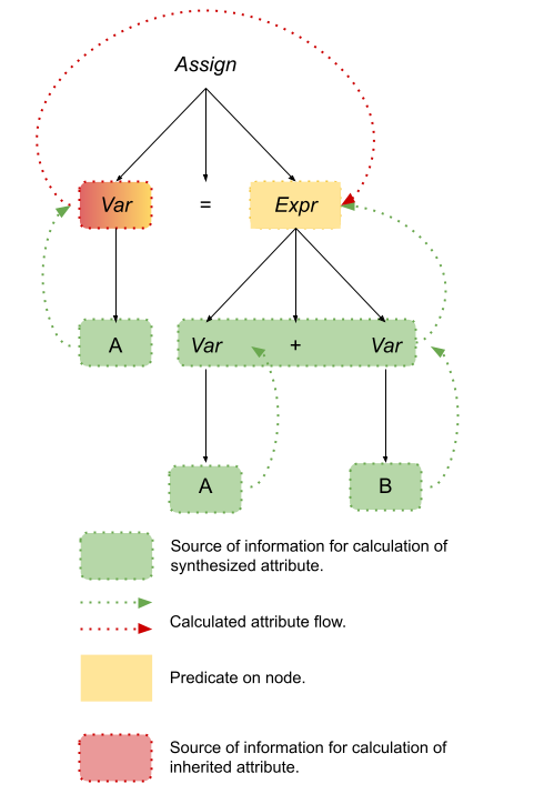
11/29/2021

Recognizing vs Generating

We have talked at length about how, depending on your vantage point, you can look at predicates in Prolog as either declarative or procedural. Viewed from a declarative perspective, the predicates will generate all the values of a variable that will make the predicate true. Viewed from the other direction, predicates look more like traditional boolean-valued functions in a procedural (or OOP) programming language. The dichotomy between the declarative and procedural view has parallels in syntax and grammars. From one end of the PL football stadium, grammars are generators; from the other endzone they are recognizers.

We have seen the power of the derivation and the parse tree to generate strings that are in a language L defined by a grammar G. We can create a valid sentence in language L by repeated application of the productions in G to the sentential forms derived from G’s start symbol. Applying all the productions in all possible combinations will eventually enumerate all valid strings in the language L (don’t hold your breath for that process to finish!).

The only problem is that (with one modern exception ), our compilers don’t actually generate source code for us! It is the programmer – us! – who writes the source code and the compiler that checks whether it is a valid program. There are obviously myriad ways in which a programmer can write an invalid program in a particular programming language and the compiler can detect all of them. However, the easiest invalid programs for the compiler to detect are the ones that are not syntactically correct.

To reiterate, (most) programming languages specify their syntax using a (context-free) grammar (CFG) – the theoretical language L that we’ve talked about as being defined by a grammar G can actually be a programming language! Therefore, the source code for a program is technically just a particular sequence of terminals from L’s alphabet. For that sequence of terminals to be a valid program, it must be the final sentential form in some derivation following the productions of G.

In other words, the compiler is not a generator but rather a recognizer.

Parsers

Recall from Chapter 2 of Sebesta (or earlier programming courses), the stages of compilation. The stage/tool that recognizes whether a particular sequence of terminals from a language’s alphabet is a valid program or not (the recognizer) is called parsing/a parser. Besides recognizing whether a program is valid, parsers convert the source code for a program written in a particular programming language defined according to a specific grammar into a parse tree.

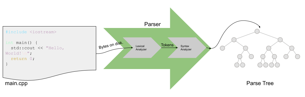
What’s sneaky is that the parsing process is really two processes: lexical analysis and syntax analysis. Lexical analysis turns the bytes on the disk into a sequence of tokens (and associated lexemes). Syntax analysis turns the tokens into a parse tree.

We’ve seen several examples of languages defined by grammars and those grammars contain productions, terminals and nonterminals. We haven’t seen any tokens, though, have we? Well, tokens are an abstract way to represent groups of bytes in a file of source code in an abstract manner. The actual bytes that are in a group that are bundled together stay associated with the token and are known as lexemes. Tokenizing the input makes the syntax analysis process easier. Note: Read Sebesta’s discussion about the reason for separating lexical analysis from syntax analysis in Section 4.1 on (approximately pg. 143). Turtles All The Way Down

Remember the Chomsky Hierarchy of languages? Context-free languages can be described by CFGs. Slightly less complex languages are known as regular languages. Regular languages can be recognized by a logical apparatus known as a finite automata (FA). If you have ever written a regular expression then you have actually written a stylized FA. Cool, right?? You will learn more about FAs in CS4040, but for now it’s important to know the broad outlines of the definition of an FA because of the central role they play in lexical analysis. An FA is

A (finite) set of states, S;
A (finite) alphabet, A;
A transition function, \(f : S, A \rightarrow S\), that takes two parameters (the current state [an element in S] and an element from the alphabet) and returns a new state;
A start state (one of the states in S); and
A set of accepting states (a subset of the states in S).

Why does this matter? Because we can describe how to group the bytes on disk into tokens (and lexemes) using regular languages. You probably have a good idea about what is going on, but let’s dig in to an example – that’ll help!

Lexical Analysis of Mathematical Expressions

For the remainder of this edition, let’s go back to the (unambiguous) grammar of mathematical expressions:

Here’s a syntactically correct expression with labeled tokens and lexemes:

What do you notice? Well, the first thing that I notice is that in most cases, the lexeme value is actually, completely, utterly useless. For instance, what other logical grouping of bytes other than the one that represents the ) will be converted in to the CLOSE_PAREN token?

There is, however, one token whose lexeme is very important: the Id token. Why? Because that token can be any number! The actual lexeme of that Id makes a big difference when it comes time to actually evaluate the mathematical expression that we are parsing (if that is, indeed, the goal of the operation!).

Certitude and Finitude

Let’s take a stab at defining the FA that we can use to convert a stream of bytes on disk in to a stream of tokens (and associated lexemes). Let yourself slip in to a world where you are nothing more than a robot with a simple memory: you can be in one of two states. Depending on the state that you are in, you are able to perform some specific actions depending on the next character that you see. The two states are BEGIN and NUMBER. When you are in the BEGIN state and you see a ), +, *, or ( then you simply emit the appropriate token and stay in the BEGIN state. If you are in the BEGIN state and you see a digit, you simply store that digit and then change your state to NUMBER. When you are in the NUMBER state, if you see a digit, you store that digit after all the digits you’ve previously seen and stay in the same state. However, when you are in the NUMBER state and you see a ), +, *, or (, you must perform three actions:

Convert the string of digits that you are remembering into a number and emit a Id token with the converted value as the lexeme;
Emit the token appropriate to the value you just saw; and
Reset your state to BEGIN.

For as long as there are bytes in the input file, you continue to perform those operations robotically. The operations that I just described are the FA’s state transition function! See how each operation depends on the current state and an input? Those are the parameters to the state transition function! And see how we specified the state we will be in after considering the input? That’s the function’s output! Woah!

What’s amazing about all those words that I just wrote is that they can be turned into a picture that is far easier to understand:

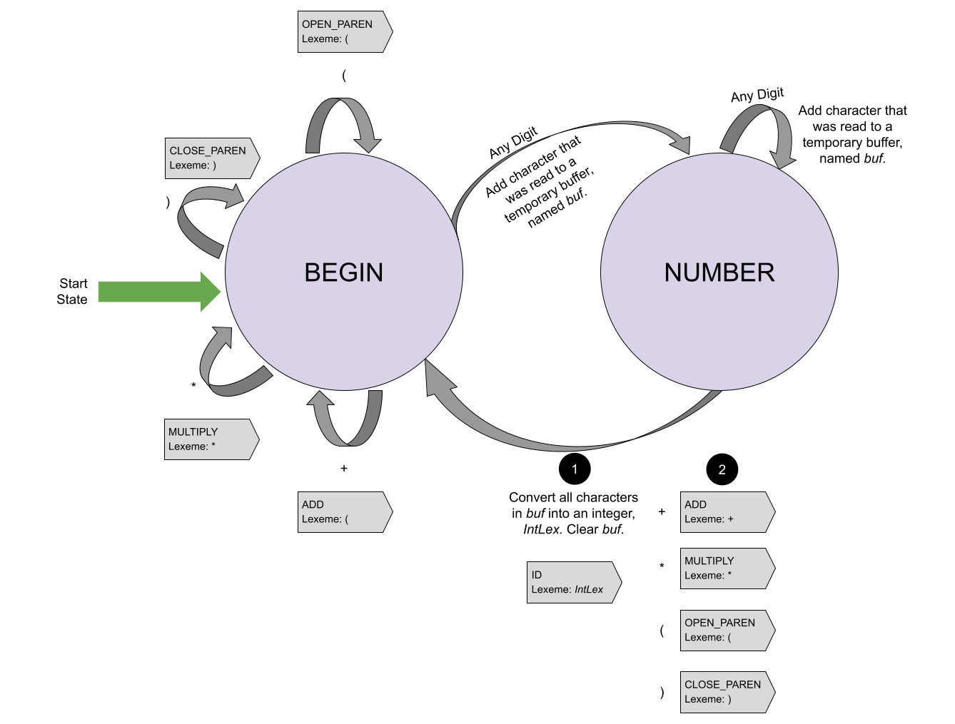
Make the connection between the different aspects of the written and graphical description above and the formal components of an FA, especially the state transition function. In the image above, the state transition function is depicted with the gray arrows!

The Last Step…

There’s just one more step … we want to convert this high-level description of a tokenizer into actual code. And, we can! What’s more, we can use a technique we learned earlier this semester in order to do it! Consider that the tokenizer will work hand-in-hand with the syntax analyzer. As the syntax analyzer goes about its business of creating a parse tree, it will occasionally turn to the lexical analyzer and say, “Give me the next token!”. In between answers, it would be helpful if the tokenizer could maintain its state.

If that doesn’t sound like a coroutine, then I don’t know what does! Because a coroutine is dormant and not dead between invocations, we can easily program the tokenizer as a coroutine so that it remembers its state (either BEGIN or NUMBER) and other information (like the current digits that it is has seen [if it is in the NUMBER state] and the progress it has made reading the input file). Kismet!

To see such an implementation in Python, check here (Links to an external site.).

12/1/2021

Peanut Butter and Jelly

To reiterate, the goal of a parser is to convert the source code for a program written in a particular programming language defined according to a specific grammar into a parse tree. Parsing occurs in two parts: lexical analysis and syntax analysis. The lexical analyzer (what we studied in the previous lecture) converts the program’s source code (in the form of bytes on disk) into a sequence of tokens. The syntax analyzer, the subject of this lecture, turns the sequence of tokens in to a parse tree. The lexical analyzer and the syntax analyzer go hand-in-hand: As the syntax analyzer goes about its business of creating a parse tree, it will periodically turn to the lexical analyzer and say, “Give me the next token!”.

We saw algorithms for building a lexical analyzer directly from the language’s CFG. It would be great if we had something similar for the syntax analyzer. In today’s lecture we are going to explore just one of the many techniques for converting a CFG into code that will build an actual parse tree. There are many such techniques, some more general and versatile than others. Sebesta talks about several of these. If you take a course in compiler construction you will see those general techniques defined in detail. In this class we only have time to cover one particular technique for translating a CFG into code that constructs parse trees and it only works for a subset of all grammars.

With those caveats in mind, let’s dig in to the details!

Descent Into Madness

A recursive-descent parser is a type of parser that can be written directly from the structure of a CFG – as long as that CFG meets certain constraints. In a recursive descent parser built from a CFG G, there is a subprogram for every nonterminal in G. Most of these subprograms are recursive. A recursive-descent parser builds a parse tree from the top down, meaning that it begins with G’s start symbol and attempts to build a parse tree that represents a valid derivation whose final sentential form matches the program’s tokens. There are other parsers that work bottom up, meaning that they start by analyzing a sentential form made up entirely of the program’s tokens and attempt to build a parse tree that that “reduces” to the grammar’s start symbol. That the subprograms are recursive and that the parse tree is built top down, the recursive-descrent parser is aptly named.

We mentioned before that there are limitations on the types of languages that a recursive-descent parser can recognize. In particular, recursive-descent parsers can only recognize LL grammars. Those are grammars whose parse trees represent a leftmost derivation and can be built from a single left-to-right scan of the input tokens. To be precise, the first L represents the left-to-right scan of the input and the second L indicates that the parser generates a leftmost derivation. There is usually another restriction – how many lookahead tokens are available. A lookahead token is the next token that the lexical analyzer will return as it scans through the input. Limiting the number of lookahead tokens reduces the memory requirements of the syntax analyzer but restricts the types of languages that those syntax analyzers can recognize. The number of lookahead tokens is written after LL and in parenthesis. LL(1) indicates 1 token of lookahead. We will see the practical impact of this restriction later in this edition.

All of these words probably seem very arbitrary, but I think that an example will make things clear!

Old Faithful

Let’s return to the grammar for mathematical expressions that we have been examining throughout this module:

We will assume that there are appropriately named tokens for each of the terminals (e.g, the ) token is CLOSE_PAREN) and that any numbers are tokenized as ID with the lexeme set appropriately.

According to the definition of a recursive-descent parser, we want to write a (possibly recursive) subprogram for each of the nonterminals in the grammar. The job of each of these subprograms is to parse the the upcoming tokens into a parse tree that matches the nonterminal. For example, the (possibly recursive) subprogram for Expr, Expr, parses the upcoming tokens into a parse tree for an expression and returns that parse tree. To facilitate recursive calls among these subprograms, each subprogram returns the root of the parse tree that it builds. The parser begins by invoking the subprogram for the grammar’s start symbol. The return value of that function call will be the root node of the parse tree for the entire input expression. Any recursive calls to other subprograms from within the subprogram for the start symbol will return parts of that overall parse tree.

I am sure that you see why each of the subprograms usually contains some recursive function calls – the nonterminals themselves are defined recursively.

How would we write such a (possibly recursive) subprogram to build a parse tree rooted at a Factor from a sequence of tokens?

There are two productions for a Factor so the first thing that the Factor subprogram does is determine whether it is parsing, for example, (5+2) – a parenthesized expression – or 918 – a simple ID. In order to differentiate, the function simply consults the lookahead token. If that token is an open parenthesis then it knows that it is going to be evaluating the production Factor \(\rightarrow ( Expr )\). On the other hand, if that token is an ID, then it knows that it is going to be evaluating the production Factor \(\rightarrow\) id. Finally, if the current token is neither an open parenthesis nor an ID, then that’s an error!

Let’s assume that the current token is an open parenthesis. Therefore, Factor knows that it should be parsing the production Factor \(\rightarrow ( Expr )\). Remember how we said that in a recursive-descent parser, each nonterminal is represented by a (possibly recursive) subprogram? Well, that means that we can assume there is a subprogram for parsing an Expr (though we haven’t yet defined it!). Let’s call that mythical subprogram Expr. As a result, the Factor subprogram can invoke Expr which will return a parse tree rooted at that expression. Pretty cool! Before continuing to parse, Factor will check Expr’s return value – if it is an error node, then parsing stops and Factor simply returns that error.

Otherwise, after successfully parsing an expression (by invoking Expr) the parser expects the next token to be a close parenthesis. So, Factor checks that fact. If everything looks good, then Factor simply returns the node generated by Expr – there’s no need to generate another node that just indicates an expression is wrapped in parenthesis. If the token after parsing the expression is not a close parenthesis, then Factor returns an error node.

Now, what happens if the lookahead token is an ID? That’s simple – Factor will just generate a node for that ID and return it!

Finally, if neither of those is true, Factor simply returns an error node.

Let’s make this a little more concrete by writing that in pseudocode. We will assume the following are defined:

Node(T, X, Y, Z …): A polymorphic function that generates an appropriately typed node (according to T) in the parse tree that “wraps” the tokens X, Y, Z, etc. We will play fast and loose with this notation.
Error(X): A function that generates an error node because token X was unexpected – an error node in the final parse tree will generate a diagnostic message.
tokenizer(): A function that returns and consumes the next token from the lexical analyzer.
lookahead(): A function that returns the lookahead token.

def Factor:
  if lookhead() == OPEN_PAREN:
    # Parsing a ( Expr )
    #
    # Eat the lookahead and move forward.
    curTok = nextToken()
    # Build a parse tree rooted at an expression,
    # if possible.
    nestedExpr = Expr()
    # There was an error parsing that expression;
    # we will return an error!
    if type(nestedExpr) == Error:
      return nestedExpr
    # Expression parsing went well. We expect a )
    # now.
    if lookahead() == CLOSE_PAREN:
      # Eat that close parenthesis.
      nextToken()
      # Return the root of the parse tree of the
      # nested expression.
      return nestedExpr
    else:
      # We expected a ) and did not get it.
      return Error(lookahead())
  else if lookahead() == ID:
    # Parsing a ID
    #
    curTok = nextToken()
    return Node(curTok)
  else:
    # Parsing error!
    return Error(lookahead())

Writing a function to parse a Factor is relatively straightforward. To get a sense for what it would be like to parse an expression, let’s write a part of the Expr subprogram:

def Expr:
  ...
    leftHandExpr = Expr()
    if type(leftHandExpr) == Error:
      return leftHandExpr
    if lookahead() != PLUS:
      curTok = nextToken()
      return Error(curTok)
    rightHandTerm = Term()
    if type(rightHandTerm) == Error:
      return rightHandTerm
    return Node(Expr, leftHandExpr, rightHandTerm)
  ...

What stands out is an emerging pattern that each of the subprograms will follow. Each subprogram is slowly matching the items from the grammar with the actual tokens that it sees. The subprogram associated with each nonterminal parses the nonterminals used in the production, “eats” the terminals in those same productions and converts it all into nodes in a parse tree. The subprogram that calls subprograms recursively melds together their return values into a new node that will become part of the overall parse tree, one level up.

We Are Homefree

I don’t know about you, but I think that’s pretty cool – you can build a series of collaborating subprograms named after the nonterminals in a grammar that call each other and, bang!, through the power of recursion, a parse tree is built! I think we’re done here.

Or are we?

Look carefully at the definition of Expr given in the pseudocode above. What is the name of the first subprogram that is invoked? That’s right, Expr. When we invoke Expr again, what is the first subprogram that is invoked? That’s right, Expr again. There’s no base case – this spiral will continue until there is no more space available on the stack!

It seems like we may have run head-on into a fundamental limitation of recursive-descent parsing: The grammars that it parses cannot contain productions that are left recursive. A production A \(\rightarrow \ldots\) is (indirect) left recursive “when A derives itself as its leftmost symbol using one or more derivations.” In other words, \(A \rightarrow^{+} A \ldots \) is indirectly recursive where \(\rightarrow^{+} \)indicates one or more productions. For example, the production for A in grammar

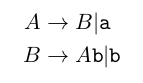
is indirect left recursive because A → B → A \mathtt{b}.

A production A \(\rightarrow \ldots \)is direct left recursive when A derives itself as its leftmost symbol using one derivation (e.g., \(A \rightarrow A \ldots\). The production for Expr in our working example is direct left recursive.

What are we to do?

Note: The definitions of left recursion are taken from:

Allen B Tucker and Robert Noonan. 2006. Programming Languages (2nd. ed.). McGraw-Hill, Inc., USA.

Formalism To The Rescue

Stand back, we are about to deploy math!

There is an algorithm for converting productions that are direct-left recursive into productions that generate the same languages and are not direct-left recursive. In other words, there is hope for recursive-descent parsers yet! The procedure is slightly wordy, but after you see an example it will make perfect sense. Here’s the overall process:

\(A \rightarrow \beta_{1}A’ | \beta_{2}A’ | \ldots | \beta_{n}A’ \\ A’ \rightarrow \alpha_{1}A’ | \alpha_{2}A’ | \ldots | \alpha_{n}A’ | \varepsilon\)

where \(\varepsilon\) is the erasure rule and matches an empty token.

I know, that’s hard to parse (pun intended). An example will definitely make things easier to grok:

\(Expr \rightarrow Expr + Term | Term\)

A is Expr, \(\alpha_1is + Term, \beta_1 is Term\). Therefore,

A \(\rightarrow \beta_{1}A’ \\ A’ \rightarrow \alpha_{1}A’ | \varepsilon \)

becomes

\(Expr \rightarrow Term Expr’ \\ Expr’ \rightarrow +TermExpr’ | \varepsilon\)

No sweat! It’s just moving pieces around on a chessboard!

The Final Countdown

We can make those same manipulations for each of the productions in the grammar in our working example and we arrive here:

\(\mathit{Expr} \rightarrow \mathit{Term}\mathit{Expr’} \\ \mathit{Expr’} \rightarrow + \mathit{Term}\mathit{Expr’} | \epsilon \\ \mathit{Term} \rightarrow \mathit{Factor}\mathit{Term’} \\ \mathit{Term’} \rightarrow * \mathit{Factor}\mathit{Term’} | \epsilon \\ \mathit{Factor} \rightarrow ( \mathit{Expr} ) | \mathit{id}\)

Now that we have a non direct-left recursive grammar we can easily write a recursive-descent parser for the entire grammar. The source code is available online and I encourage you to download and play with it!

10/1/2021