10/15/2021
The hunt for October!
Corrections
None to speak of!!
Introduction to Functional Programming
We spent Friday beginning our module on Functional Programming (FP)! As we said at the beginning of the semester when we were learning about programming paradigms, FP is very different than imperative programming. In imperative programming, developers tell the computer how to do the operation. While functional programming is not logic programming (where developers just tell the computer what to compute and leave the how entirely to the language implementation), the writer of a program in a functional PL is much more concerned with specifying what to compute than how to compute it.

Four Characteristics of Functional Programming
There are four characteristics that epitomize FP:
- There is no state
- Functions are central
- Functions can be parameters to other functions
- Functions can be return values from other others
- Program execution is function evaluation
- Control flow is performed by recursion and conditional expressions
- Lists are a fundamental data type
In a functional programming language, there are no variables, per se. And because there are no variables, there is no state. That does not mean there are no names. Names are still important. It simply means that names refer to expressions themselves and not their values. The distinction will become more obvious as we continue to learn more about writing programs in functional languages.
Because there is no state, a functional programming language is not history sensitive. A language that is history sensitive means that results of operations in that language can be affected by operations that have come before it. For example, in an imperative programming language, a function may be history sensitive if it relies on the value of a global variable to calculate its return value. Why does that count as history sensitive? Because the value in the global variable could be affected by prior operations.
A language that is not history sensitive has referential transparency. We learned the definition of referential transparency before, but now it might make a little more sense. In a language that has referential transparency, a the same function called with the same arguments generates the same result no matter what operations have preceded it.
In a functional programming language there are no loops (unless they are added as syntactic sugar) – recursion is the way to accomplish repetition. Selective execution (as opposed to sequential execution) is accomplished using the conditional expression. A conditional expression is, well, an expression that evaluates to one of two values depending on the value of a condition. We have seen conditional expressions in STIMPL. That a conditional statement can have a value (thus making it a conditional expression) is relatively surprising for people who only have experience in imperative programming languages. Nevertheless, the conditional expressions is a very, very sharp sword in the sheath of the functional programmer.
A functional program is a series of functions and the execution of a functional program is simply an evaluation of those functions. That sounds abstract at this point, but will become more clear when we see some real functional programs.
Lists are a fundamental data type in functional programming languages. Powerful syntactic tools for manipulating lists are built in to most functional PLs. Understanding how to wield these tools effectively is vital for writing code in functional PLs.
The Historical Setting of the Development of Functional PLs
The first functional programming language was developed in the mid-1950s by John McCarthy . At the time, computing was most associated with mathematical calculations. McCarthy was instead focused on artificial intelligence which involved symbolic computing. Computer scientists thought that it was possible to represent cognitive processes as lists of symbols. A language that made it possible to process those lists would allow developers to build systems that work like our brains.

McCarthy started with the goal of writing a system of meta notation that programmers could attach to Fortran. These meta notations would be reduced to actual Fortran programs. As they did their work, they found their way to a program representation built entirely of lists (and lists of lists, and lists of lists of lists, etc). Their thinking resulted in the development of Lisp, a list processing language. In Lisp, data are lists and programs are lists. They showed that list processing, the basis of the semantics of Lisp, is capable of universal computing. In other words, Lisp, and other list processing languages, is/are Turing complete.
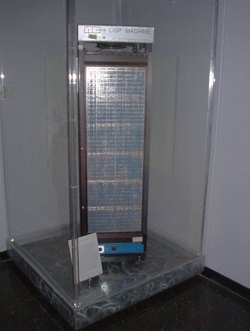
The inability to execute a Lisp program efficiently on a physical computer based on the von Neumann model has given Lisp (and other functional programming languages) a reputation as slow and wasteful. (N.B.: This is not true today!) Until the late 1980s hardware vendors thought that it would be worthwhile to build physical machines with non-von Neumann architectures that made executing Lisp programs faster. Here is an image of a so-called Lisp Machine.
LISP
We will not study Lisp in this course. However, there are a few aspects of Lisp that you should know because they pervade the general field of computer science.
First, you should know CAR, CDR and CONS – pronounced car, could-er, and cahns, respectively. CAR is a function that takes a list as a parameter and returns the first element of the list. CDR is a function that takes a list as a parameter and returns the tail, everything but the head, of the list. CONS takes two parameters – a single element and a list – and returns a new list with the first argument appended to the front of the second argument.
For instance,
(car (1 2 3))
is 1.
(cdr (1 2 3))
is (2 3).
Second, you should know that, in Lisp, all data are lists and programs are lists.
(a b c)
is a list in Lisp. In Lisp, (a b c) could be interpreted as a list of atoms a, b and c or an invocation of function a with parameters b and c.
Lambda Calculus
Lambda Calculus is the theoretical basis of functional programming languages in the same way that the Turing Machine is the theoretical basis of the imperative programming languages. The Lambda Calculus is nothing like “calculus” – the word calculus is used here in its strict sense: a method or system of calculation . It is better to think of Lambda Calculus as a programming language rather than a branch of mathematics.
Lambda Calculus is a model of computation defined entirely by function application. The Lambda Calculus is as powerful as a Turning Machine which means that anything computable can be computed in the Lambda Calculus. For a language as simple as the Lambda Calculus, that’s remarkable!
The entirety of the Lambda Calculus is made up of three entities:
- Expression: a name, a function or an application
- Function: \(\lambda\)
. - Application:
Notice how the elements of the Lambda Calculus are defined in terms of themselves. In most cases it is possible to restrict names in the Lambda Calculus to be any single letter of the alphabet – a is a name, z is a name, etc. Strictly speaking, functions in the Lambda Calculus are anonymous – in other words they have no name. The name after the
in a function in the Lambda Calculus can be thought of as the parameter of the function. Here’s an example of a function in the Lambda Calculus:
\(\lambda\)x . x
Lambda Calculiticians (yes, I just made up that term) refer to this as the identity function. This function simply returns the value of its argument! But didn’t I say that functions in the Lambda Calculus don’t have names? Yes, I did. Within the language there is no way to name a function. That does not mean that we cannot assign semantic values to those functions. In fact, associating meaning with functions of a certain format is exactly how high-level computing is done with the Lambda Calculus.