11/15/2021

Red Alert

At the end of lecture on Friday, we discussed the two different types of cuts – red and green. A green cut is one that does not alter the behavior of a Prolog program. A red cut does alter the behavior of a Prolog program. The implication was that red cuts are bad and green cuts are good. But, is this always the case?

To frame our discussion, let’s look at a Prolog program that performs a Bubble Sort on a list of numbers. The predicate, bsort/2, is defined like this:

bsort(Unsorted, Sorted):-
  append(Left, [A, B | Right], Unsorted),
  B<A,
  append(Left, [B, A | Right], MoreSorted),
  bsort(MoreSorted, Sorted).
bsort(Sorted, Sorted).

The first rule handles the recursive case (when there is at least one list item out of order) and the second rule handles the base case (when the list is sorted). According to this definition, how does Prolog handle the query

bsort([2,1,3,5], M).

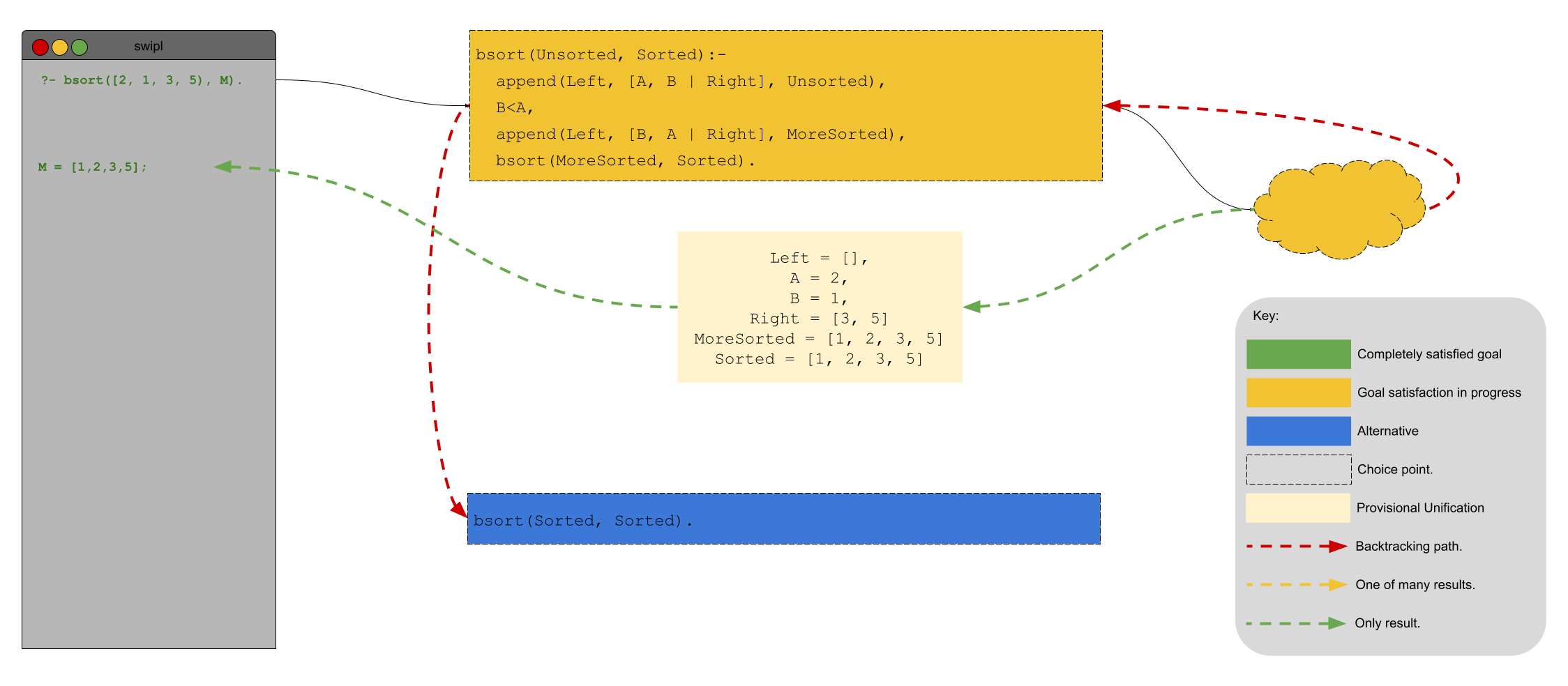
Prolog (as we are well aware) searches its rule top to bottom. The first rule that it sees is the recursive case and Prolog immediately opts for it. Opting for this case is not without consequences – a choice point is created. Why? Because Prolog made the choice to attempt to satisfy the query according to the first rule and not the (just as applicable) second rule! Let’s call this choice point A.

Next, Prolog attempts to unify the subquery append(Left, [A, B | Right], Unsorted). The first (of many) unifications that append/3 generates is Left = [], A = 2, B = 1, Right = [3, 5]. By continuing with this particular unification, Prolog creates another choice point. For what reason? Well, Prolog knows that append/3 could generate other potential unifications and it will need to check those to see if they, too, satisfy the original query! Let’s call this choice point B. Next, Prolog checks whether A is less than B – it is. Prolog continues in a like manner to satisfy the final two subgoals of the rule.

When Prolog does satisfy those, it has generated a sorted version of [2,1,3,5]. It reports that result to the querier. Great! There’s only one problem. There are still choice points that Prolog wants to explore. In particular, there are choice points A and B. In this case, we can forget about choice point B because there are no other unifications of append/3 that meet the criteria for A<B in Unsorted. In other words, visually the situation looks like this:

If the querier is using bsort/2 declaratively, this scenario is a problem: Prolog will backtrack to choice point A and then consider the base case rule for bsort/2. In other words, Prolog will also generate

[2,1,3,5]

as a unification! This is clearly not right. What’s more, the Prolog programmer could query for

bsort([3,2,1,4,5], Sorted).

in which choice point B will have consequences. Run this query for yourself (using trace), examine the results, and make sure you understand why the results are generated.

So, what are we to do? cut/0 (Links to an external site.) to the rescue! Logically speaking, once our bsort/3 rule finds a single element out of order and we adjust that element, the recursive call to itself will handle ordering any other unordered elements. In other words, we can forget any earlier choice points! This is exactly what the cut is intended for!

Let’s rewrite bsort/3 using cuts and see if our problem is sorted (see what I did there?):

bsort(Unsorted, Sorted):-
  append(Left, [A, B | Right], Unsorted),
  B<A, !,
  append(Left, [B, A | Right], MoreSorted),
  bsort(MoreSorted, Sorted).
bsort(Sorted, Sorted).

And now let’s see how our earlier troublesome queries perform:

?- bsort([2,1,3,5], Sorted).
Sorted = [1, 2, 3, 5].

?- bsort([3,2,1,4,5], Sorted).
Sorted = [1, 2, 3, 4, 5].

Amazing!

Here’s the rub: The version of our Prolog program with the cut gave different results than the version without. Is this cut a green or a red cut? That’s right, it’s a red cut. I guess there are such things as good red cuts after all!

The Fundamentals

As we have said in the past, there is a theoretical underpinning for each of the programming paradigms that we have studied this semester. Logic programming is no different. The theory behind logic programming is first-order predicate logic. Predicate logic is an extension of propositional logic. Propositional logic is based on the evaluation of propositions.

A proposition is simply any statement that can be true or false. For example,

• Will is a programmer.
• Alicia is a programmer.
• Sam is a programmer.

Those statements can be true or false. In propositional logic we can build more complicated propositions from existing propositions using logical connectives like and, or, not, and implication (if … then). Each of these has an associated truth table to determine the truth of two combined propositions.

Look closely at the example propositions above and you will notice an underlying theme: they all do with someone (let’s call them x) being a programmer. In propositional logic, our ability to reason using that underlying theme is impossible. We can only work with the truth of the statement as a whole.

If we add to propositional logic variables, constants, and quantifiers then we get predicate logic and we are able to reason more subtly. Although you might argue that propositional logic has variables, everyone can agree that they are limited – they can only have two values, true and false. In first-order predicate logic, variables can have domains other than just {T, F}. That’s already a huge step!

Quantifiers “define” variables and “constrain” their possible values. There are two quantifiers in first-order predicate logic – the universal and the existential. The universal is the “for all” (aka “every”) quantifier. We can use the universal quantifier to write statements (in logic) like “Every person is a Bearcats fan.” Symbolically, we write the universal quantifier with the \(\forall\). We can write our obvious statement from above in logic like

Now we are talking! As for the existential quantifier, it allows us to write statements (in logic) like “There is some person on earth that speaks Russian.” Symbolically, we write the existential quantifier with the \(\exists\). We can write the statement about our Russian-speaking person as

How are quantifiers embedded in Prolog? Variables in Prolog queries are existentially qualified – “Does there exist …?“​ Variables in Prolog rules are universally quantified – “For all ….”

In first-order predicate logic, there are such things as Boolean-valued functions. This is familiar territory for us programmers. A Boolean-valued function is a function that has 0 or more parameters and returns true or false.

With these definitions, we can now define predicates: A predicate is a proposition in which some Boolean variables are replaced by Boolean-valued functions and quantified expressions. Let’s look at an example.

is a proposition where p and q are boolean variables. Replace p with the Boolean-valued function \(is\_teacher(x)\) and q with the quantified expression \(\exists y(student(x) \land teaches(x, russion))\) and we have the predicate

There is only one remaining question: Why is it called first-order predicate logic and not, say, higher-order predicate logic? “First-order” here indicates that the predicates in this logic cannot manipulate or reason about predicates themselves. Does this sound familiar? Imperative languages can define functions but they cannot reason about functions themselves while functional languages can!