9/20/2021
This is an issue of the Daily PL that you are going to want to make sure that you keep safe – definitely worth framing and passing on to your children! You will want to make sure you remember where you were when you first learned about …
Formal Program Semantics
Although we have not yet learned about it (we will, don’t worry!), there is a robust set of theory around the way that PL designers describe the syntax of their language. You can use regular expressions, context-free grammars, parsers (recursive-descent, etc) and other techniques for defining what is a valid program.
On the other hand, there is less of a consensus about how a program language designer formally describes the semantics of programs written in their language. The codification of the semantics of a program written in a particular is known as formal program semantics. In other words, formal program semantics are a precise mathematical description of the semantics of an executing program. Sebesta uses the term dynamic semantics which is defines as the “meaning[] of the expressions, statements and program units of a programming language.”
The goal of defining formal program semantics is to understand and reason about the behavior of programs. There are many, many reasons why PL designers want a formal semantics of their language. However, there are two really important reasons: With formal semantics it is possible to prove that
- two programs calculate the same result (in other words, that two programs are equivalent), and
- a program calculates the correct result.
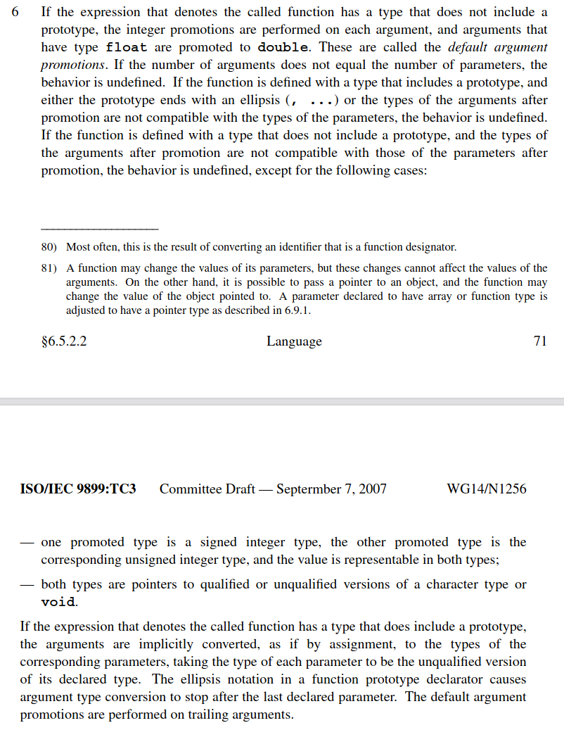
The alternative to formal program semantics are standards promulgated by committees that use natural language to define the meaning of program elements. Here is an example of a page from the standard for the C programming language:
If you are interested, you can find the C++ language standard , the Java language standard , the C language standard , the Go language standard and the Python language standard all online.
Testing vs Proving
There is absolutely a benefit to testing software. No doubt about it. However, testing that a piece of software behaves a certain way does not prove that it operates a certain way.
“Program testing can be used to show the presence of bugs, but never to show their absence!” - Edsger Dijkstra
There is an entire field of computer science known as formal methods whose goal is to understand how to write software that is provably correct. There are systems available for writing programs about which things can be proven. There is PVS, Coq ,Isabelle , and TLA+ , to name a few. PVS is used by NASA to write its mission-critical software and even it makes an appearance in the movie The Martian .
Three Types of Formal Semantics
There are three common types of formal semantics. It is important that you know the names of these systems, but we will only focus on one in this course!
- Operational Semantics: The meaning of a program is defined by how the program executes on an idealized virtual machine.
- Denotational Semantics: Program units “denote” mathematical functions and those functions transform the mathematically defined state of the program.
- Axiomatic Semantics: The meaning of the program is based on proof rules for each programming unit with an emphasis on proving the correctness of a program.
We will focus on operational semantics only!
Operational Semantics
Program State
We have referred to the state of the program throughout this course. We have talked about how statements in imperative languages can have side effects that affect the value of the state and we have talked about how the assignment statement’s raison d’etre is to change a program’s state. For operational semantics, we have to very precisely define a program’s state.
At all times, a program has a state. A state is just a function whose domain is the set of defined program variables and whose range is V * T where V is the set of all valid variable values (e.g., 5, 6.0, True, “Hello”, etc) and T is the set of all valid variable types (e.g., Integer, Floating Point, Boolean, String, etc). In other words, you can ask a state about a particular variable and, if it is defined, the function will return the variable’s current value and its type.
It is important to note that PL researchers have math envy. They are not mathematicians but they like to use Greek symbols. So, here we go:
\begin{equation*} \sigma(x) = (v, \tau) \end{equation*}
The state function is denoted with the σ . τ always represents some arbitrary variable type. Generally, v represents a value. So, you can read the definition above as “Variable x has value v and type τ in state σ.”
Program Configuration
Between execution steps (a term that we will define shortly), a program is always in a particular configuration:
\begin{equation*} <e, \sigma> \end{equation*}
This means that the program in state σ
is about to evaluate expression e.
Program Steps
A program step is an atomic (indivisible) change from one program configuration to another. Operational semantics defines steps using rules. The general form of a rule is
\begin{equation*} \frac{premises}{conclusion} \end{equation*}
The conclusion is generally written like <e, σ> ⟶ (v, τ, σ). This statement means that, when the premises hold, the rule evaluates to a value (v), type (τ) and (possibly modified) state (σ’) after a single step of execution of a program in configuration <e, σ>. Note that rules do not yield configurations. All this will make sense when we see an example.
Example 1: Defining the semantics of variable access.
In STIMPL, the expression to access a variable, say i, is written like Variable(“i”). Our operational semantic rule for evaluating such an access should “read” something like: When the program is about to execute an expression to access variable i in a state σ, the value of the expression will be the triple of i’s value, i’s type and the unchanged state σ." In other words, the evaluation of the next step of a program that is about to access a value is the value and type of the variable being accessed and the program’s state is unchanged.
Let’s write that formally!
\begin{equation*} \(\frac{\sigma(x) \rightarrow (v, \tau)} {<\text{Variable}(x), \sigma > \rightarrow (v, \tau, \sigma)}\) \end{equation*}
State Update
How do we write down that the state is being changed? Why would we want to change the state? Let’s answer the second question first: we want to change the state when, for example, there is an assignment statement. If σ (“i”) = (4, Integer) and then the program evaluated an expression like Assign(Variable(“i”), IntLiteral(2)), we don’t want the σ
function to return (4, Integer) any more! We want it to return (2, Integer). We can define that mathematically like:
\begin{equation*} \sigma[(v,\tau)/x](y)= \begin{cases} & \sigma(y) \quad y \ne x \ &(v,\tau) \quad y=x \end{cases} \end{equation*}
This means that if you are querying the updated state for the variable that was just reassigned (x), then return its new value and type (m and τ ). Otherwise, just return the value that you would get from accessing the existing σ
.
Example 2: Defining the semantics of variable assignment (for a variable that already exists).
In STIMPL, the expression to overwrite the value of an existing variable, say i, with, say, an integer literal 5 is written like Assign(Variable("i"), IntLiteral(5)). Our operational semantic rule for evaluating such an assignment should “read” something like: When the program is about to execute an expression to assign variable i to the integer literal 5 in a state σ
and the type of the variable i in state σ is Integer, the value of the expression will be the triple of 5, Integer and the changed state σ’ which is exactly the same as state σ
except where (5, Integer) replaced i’s earlier contents." That’s such a mouthful! But, I think we got it. Let’s replace some of those literals with symbols for abstraction purposes and then write it down!
\begin{equation*} \frac{<e, \sigma> \longrightarrow (v, \tau, \sigma’), \sigma(x) \longrightarrow (*,, \tau)} {<\text{Assign(Variable)}(x, e), \sigma > \longrightarrow (v, \tau, \sigma’ [(v, \tau)/x])} \end{equation*}
Let’s look at it step-by-step:
\begin{equation*} <Assign(Variable(x),e),\sigma> \end{equation*}
is the configuration and means that we are about to execute an expression that will assign value of expression e to variable x. But what is the value of expression e? The premise
\begin{equation} <e,\sigma>⟶(v,\tau, \sigma′) \end{equation}
tells us that the value and type of e when evaluated in state σ is v, and τ. Moreover, the premise tells us that the state may have changed during evaluation of expression e and that subsequent evaluation should use a new state, σ
‘. Our mouthful above had another important caveat: the type of the value to be assigned to variable x must match the type of the value already stored in variable x. The second premise
\begin{equation*} \sigma′(x)\longrightarrow(*, \tau) \end{equation*}
tells us that the types match – see how the τs are the same in the two premises? (We use the * to indicate that we don’t care what that value is!)
Now we can just put together everything we have and say that the expression assigning the value of expression e to variable x evaluates to
\begin{equation*} (v,\tau,\sigma′[(v,\tau)/x]) \end{equation*}
That’s Great, But Show Me Code!
Well, Will, that’s fine and good and all that stuff. But, how do I use this when I am implementing STIMPL? I’ll show you! Remember the operational semantics for variable access:
\begin{equation*} \(\frac{\sigma(x) \rightarrow (v, \tau)} {<\text{Variable}(x), \sigma > \rightarrow (v, \tau, \sigma)}\) \end{equation*}
Compare that with the code for it’s implementation in the STIMPL skeleton that you are provided for Assignment 1:
def evaluate(expression, state):
...

    case Variable(variable_name=variable_name):
      value = state.get_value(variable_name)
      if value == None:
        raise InterpSyntaxError(f"Cannot read from {variable_name} before assignment.")
      return (*value, state)
At this point in the code we are in a function named evaluate whose first parameter is the next expression to evaluate and whose second parameter is a state. Does that sound familiar? That’s because it’s the same as a configuration! We use pattern matching to select the code to execute. The pattern is based on the structure of expression and we match in the code above when expression is a variable access. Refer to Pattern Matching in Python for the exact form of the syntax. The state variable is an instance of the State object that provides a method called get_value (see Assignment 1: Implementing STIMPL for more information about that function) that returns a tuple of (v, τ) In other words, get_value works the same as σ. So,
value = state.get_value(variable_name)
is a means of implementing the premise of the operational semantics.
return (*value, state)
yields the final result! Pretty cool, right?
Let’s do the same analysis for assignment:
\(\frac{<e,\sigma>\longrightarrow(v,\tau,\sigma′),\sigma′(x)\longrightarrow(*,\tau)}{<Assign(Variable(x),e),σ>\longrightarrow(v,\tau,σ′[(v,\tau)/x])}\)
And here’s the implementation:
def evaluate(expression, state):
...

   case Assign(variable=variable, value=value):

      value_result, value_type, new_state = evaluate(value, state)

      variable_from_state = new_state.get_value(variable.variable_name)
      _, variable_type = variable_from_state if variable_from_state else (None, None)

      if value_type != variable_type and variable_type != None:
        raise InterpTypeError(f"""Mismatched types for Assignment:
            Cannot assign {value_type} to {variable_type}""")

      new_state = new_state.set_value(variable.variable_name, value_result, value_type)
      return (value_result, value_type, new_state)
First, look at
value_result, value_type, new_state = evaluate(value, state)
which is how we are able to find the values needed to satisfy the left-hand premise. value_result is v, value_type is τ and new_state is σ’.
variable_from_state = new_state.get_value(variable.variable_name)
is how we are able to find the values needed to satisfy the right-hand premise. Notice that we are using new_state (σ’) to get variable.variable_name (x). There is some trickiness in_, variable_type = variable_from_state if variable_from_state else (None, None) to set things up in case we are doing the first assignment to the variable (which sets its type), so ignore that for now! Remember that in our premises we guaranteed that the type of the variable in state σ’ matches the type of the expression:
      if value_type != variable_type and variable_type != None:
        raise InterpTypeError(f"""Mismatched types for Assignment:
            Cannot assign {value_type} to {variable_type}""")
performs that check!
new_state = new_state.set_value(variable.variable_name, value_result, value_type)
generates a new, new state (σ′[(v,τ)/x]) and
return (value_result, value_type, new_state)
yields the final result!